Tag: pivot table style

There are many built-in PivotTable styles in Excel 2007, but you might not see one that has the exact formatting you need. For example, you might like the heading colors in the Pivot Style Medium 9, but you’d like a different color in the subtotal row.

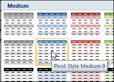
Instead of using one of the built-in PivotTable styles, you can create a custom PivotTable style with the formatting you prefer. You can either duplicate an existing Pivot Table style, and modify the duplicate, or you can create a new style from scratch.

Copy an Existing PivotTable Style

If you find a PivotTable style that’s close to what you need, you can duplicate that style, and modify the duplicate. Follow these steps to create a custom style, based on an existing style:

1. Select a cell in the pivot table, and on the Ribbon, click the Design tab.
2. In the PivotTable Styles gallery, right-click the style you want to duplicate.
3. In the context menu, click Duplicate.

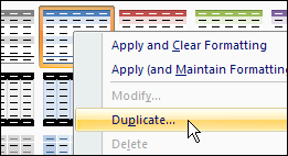
Next, follow the steps in the Modify the PivotTable Style section (below), to name and modify the new style.

Create a New PivotTable Style From Scratch

If you don’t see anything similar to what you need, you can create a new style from scratch. Follow these steps to create a new style.

1. Select a cell in the pivot table, and on the Ribbon, click the Design tab.
2. In the PivotTable Styles gallery, click New PivotTable Style (at the bottom of the PivotTable Styles gallery)

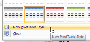
Next, follow the steps in the Modify the PivotTable Style section (below), to name and modify the new style.

Modify the PivotTable Style

After duplicating or creating a PivotTable style, follow these steps to name the style and set the formatting.

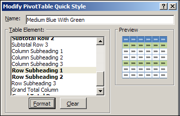
1. In the Modify PivotTable Quick Style dialog box, type a name for the new PivotTable style. (If you created a new style, the dialog box will be named New PivotTable Quick Style.)
2. To modify an element’s formatting, click it to select it, and then click the Format button. (Note: In the Table Element list, the elements in bold font have formatting applied. You can modify or clear that formatting. You can also select unformatted elements and format them.)
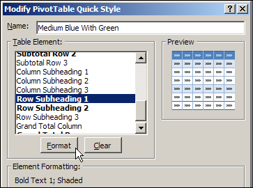
3. In the Format Cells dialog box, select the Font, Border, and Fill settings you want for the selected element.
4. Click OK, to return to the New PivotTable Quick Style dialog box, where the formatted element is listed with a bold font. In the screenshot below, you can see the revised color in the Preview section.
5. Repeat Steps 2 to 4, for any other elements that you want to format.
6. (optional) If you want your custom style to be the default PivotTable style, add a check mark to Set As Default PivotTable Quick Style For This Document.
7. Click OK, to close the New PivotTable Quick Style dialog box.

Apply the Custom PivotTable Style

The new PivotTable style that you created will not be automatically applied to the active pivot table. Follow these steps to apply your custom style.

1. Select a cell in the pivot table that you want to format.
2. Open the PivotTable Styles gallery.
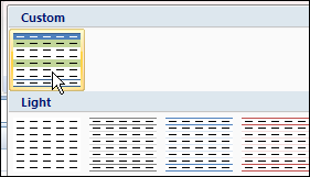
3. The custom PivotTable Style you created is added to a Custom section at the top of the PivotTable Styles gallery.
4. Click your custom style, to apply it to the active pivot table.

__________