Create Two Pivot Tables on Excel Worksheet

In a comment on this blog, someone asked how to create two pivot tables on the same Excel worksheet.

NOTE: See the updated version of this Two Pivot Tables article, from July 2020.

Shown below is a worksheet named Pivot_Reports, with a pivot table on it, based on the data on the Sales_East sheet.
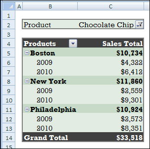
TwoPT01

We’ll add another pivot table to the Pivot_Reports sheet, based on data on the Sales_North sheet.

Add the Second Pivot Table

  • Select the Sales_North sheet, and select a cell in the data table.
  • On the Ribbon, click the Insert tab
  • In the Tables group, click PivotTable (click the top half of the PivotTable command).

RibbonInsertPT

  • In the Create PivotTable dialog box, at the top, leave the default selection of Select a Table or Range, where the Sales_North table shows.
  • In the lower section, click Existing Worksheet.
  • Click in the Location box, then click on the sheet tab for the Pivot_Reports sheet.
  • Click on the cell where the second pivot table should start.

TwoPT02

  • Click OK to create the new pivot table.
  • Add the fields that you’d like in the new pivot table.

The second pivot table is added to the Pivot_Reports worksheet.
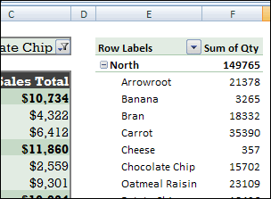
TwoPT03

Prevent Pivot Table Overlap

When you have two or more pivot tables on the same worksheet, be careful to prevent them from overlapping.

PTOverlap

Before you add new fields to the pivot table on the left, you might have to add blank columns between the pivot tables. Or, if one pivot table is above the other, add blank rows between them.

If the pivot tables will change frequently, adding and removing fields, it may be better to keep the pivot tables on separate sheet.

This short video shows pivot table refresh problems, and how to avoid them. For detailed written notes, go to the Pivot Table Errors page on my Contextures site.

Related Articles

Create a Pivot Table In Excel

Create Two Pivot Tables On Excel Worksheet

____________

Create Multiple Subtotals in a Pivot Table

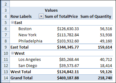
When you add multiple fields to the Row Labels area in a pivot table, subtotals automatically appear for the outer fields. In the pivot table shown below, Region and City fields are in the Row Labels area. Two fields are in the Values area: Sum of Quantity shows the total quantity for each city, and Sum of TotalPrice shows the total sales amount.

MultiSub01

Region Subtotal is Shown

A subtotal row is at the bottom of each region. It shows the total quantity and total sales for each region. You can add another row of subtotals for each region, to show the average quantity and sales. 

Add More Subtotals

You can change the field settings for the Region field and it will show more subtotal rows:

  1. Right-click one of the Region row labels, and click Field Settings.

    FieldSettings

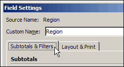
  2. In the Field Settings dialog box, click the Subtotals & Filters tab.

    FieldSettingsSF

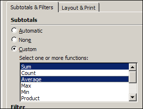
  3. In the Subtotals section, click Custom. Note: When you select Custom, the Automatic subtotal is removed.
  4. In the list of functions, click Sum and Average – the functions you want to use as subtotals. 

    FieldSettingsSub

  5. Click OK, to close the Field Settings dialog box

Note: When you select multiple Custom subtotals, the subtotals are displayed at the bottom of the group, even if you set the option to show subtotals at the top of the group.

_________________

Change the Series Order in a Pivot Chart

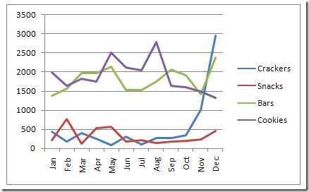
When you create a pivot chart, the series order is automatically applied. In this example, the product categories had been manually sorted in the pivot table. In the pivot chart legend, the products are in the same order: Crackers, Snacks, Bars and Cookies.

ChartSeries01

In a longer list of items, you might like the series sorted alphabetically, so they’re easier to find in the list.

Change the Sort Order

To change the sort order, follow these steps:

  1. Select the pivot chart
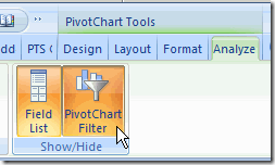
  2. If the PivotChart Filter pane isn’t visible, click the Analyze tab on the Ribbon, then click PivotChart Filter.RibbonPivotChartFilter
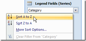
  3. In the PivotChart Filter pane, click the arrow in the drop-down list for the field you want to sort. In this example,
    click the arrow for the Legend Fields (series), where the Category field is listed.ChartSeries02
  4. Click Sort A-Z, to sort the categories in ascending order

ChartSeries03

Pivot Table Series Order

NOTE: Changing the series order in the Pivot Chart will also affect the Pivot Table on which it is based.

_________________

Hide Error Values in Pivot Table

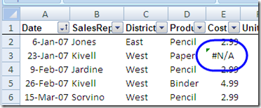
Sometimes there are errors in the source data on which a pivot table is based. For example, in the screen shot below, there is an #N/A error in the Cost column of the list.

ErrorWksht

Show or Hide Errors?

In most cases, I like to see the errors on the worksheet, so that source data problems are easy to spot.

However, you might prefer to hide the errors in the pivot table, instead of showing them there.

Open PivotTable Options

By default, error values are displayed in a pivot table.

However, by changing the PivotTable Options, you can hide the errors, so blank cells appear instead of the errors.

To hide the errors, follow these steps:

  • Right-click any cell in the pivot table
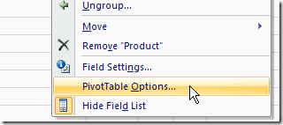
  • Next, in the pop-up context menu, click PivotTable Options.

PTOptions

Change Error Setting

When the PivotTable Options window opens, follow these steps:

  • First, in the PivotTable Options dialog box, click the Layout & Format tab.
  • Next, in the Format section, add a check mark to “For Error Values Show”.

PTErrorVal

Specify Error Value Text

In the box beside the  “For Error Values Show” setting, you can specify what text to use, to replace any error.

  • Blank: If you leave the text box blank, the errors will be replaced with blank cells.
  • Text: You can type one or more characters, such as a hyphen, or “NA”, to replace the error values with that text.

After you finish your change to the For Error Values Show setting:

  • Click the OK button, to close the PivotTable Options dialog box.

Note: Values Area Only

  • This pivot table option setting only affects cells in the Values area of the pivot table.
  • If error values appear in the Row Labels, Column Labels, or Report Filter area, they will not be replaced.

_____________________

Allow Excel Pivot Table Use on Protected Sheet

In some workbooks, you might want to allow users to make changes to a pivot table, but you need to protect formulas or data in other areas of the worksheet.

If you protect the worksheet and enable pivot table use, users will be able to modify the pivot table, but won’t have access to other locked parts of the worksheet.

Prepare the Worksheet

The first step is to unlock cells where changes can be made. Then, turn on the worksheet protection.

  1. Select any cells in which users are allowed to make changes. In this example, users can make changes to cell E2.
  2. On the Ribbon, click the Home tab.
  3. In the Cells group, click Format. If the Lock Cell command is enabled, click Lock Cell to unlock the selected cell.LockCell

Protect the Worksheet

Next, protect the worksheet:

  • On the Ribbon, click the Review tab, and in the Changes section, click Protect Sheet.

ProtectSheet

  • If desired, enter a password.
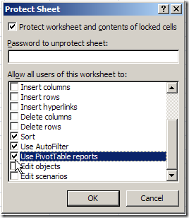
  • Add a check mark to Use PivotTable reports, and check any other items you want enabled on the protected worksheet.

UsePivotTableReportsOn

  • Click OK and confirm the password, if you entered one.

Test the Worksheet

Because the worksheet is protected, and Use PivotTable Reports was selected, users will be able to make changes to the pivot table. For example, they will be able to move fields, add fields, and use the drop-down lists.

However, some pivot table features won’t be available while the worksheet is protected, including:

  • Refresh
  • Group and Ungroup
  • Report Layout
  • Calculated Field

Other pivot tables, based on the same Excel Table as the pivot tables on a protected sheet, will have some features disabled, such as Refresh.

Tip: To refresh a pivot table on a protected sheet, temporarily unprotect the worksheet, refresh the pivot table, and then protect the sheet.

Watch the Video

In this short video, you can see the step by step instructions for preparing and protecting the worksheet.

_____________________


Block Excel Pivot Table on Protected Sheet

In some workbooks, you might want to prevent users from making any changes to a pivot table. You want them to see the pivot table, but not change it. However, users might need to make changes to data in other areas of the worksheet.

If you protect the worksheet without enabling pivot table use, users won’t be able to modify the pivot table, but will have access to other unlocked parts of the worksheet.

Prepare the Worksheet

The first step is to unlock cells where changes can be made. Then, turn on the worksheet protection.

  • Select any cells in which users are allowed to make changes. In this example, users can make changes to cell E2.
  • On the Ribbon, click the Home tab.
  • In the Cells group, click Format. If the Lock Cell command is enabled, click Lock Cell to unlock the selected cell.

LockCell

Protect the Worksheet

Next, protect the worksheet:

  • On the Ribbon, click the Review tab, and in the Changes section, click Protect Sheet.

ProtectSheet

  • If desired, enter a password.
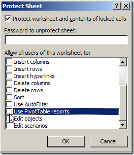
  • Remove the check mark for Use PivotTable reports, and check any other items you want enabled on the protected worksheet.

UsePivotTableReportsOff

  • Click OK and confirm the password, if you entered one.

Test the Worksheet

Because the worksheet is protected, and Use PivotTable Reports was not selected, users won’t be able to make changes to the pivot table, and the field list will be hidden.

NOTE: Other pivot tables, based on the same Excel Table as the pivot tables on a protected sheet, will have some features disabled, such as Refresh.

Tip: To refresh a pivot table on a protected sheet, temporarily unprotect the worksheet, refresh the pivot table, and then protect the sheet.

Watch the Video

In this short video, you can see the step by step instructions for preparing and protecting the worksheet.

_____________________


Create an Excel Table in Excel 2007

An Excel Table is a new feature in Excel 2007, similar to the List feature in Excel 2003. An Excel Table makes it easy for you to sort, filter, and review your data, whether it’s a few rows and columns, or thousands.

You can also use an Excel Table as the source for a Pivot Table, and new data will automatically be included in the Pivot Table source.

Arrange Your Data

Prepare your data before creating an Excel Table:

  • Enter your data on a worksheet, in rows and columns, with headings in the first row.
  • Remove any blank rows or columns within the data
  • Leave at least one blank row and one blank column between your data, and any other data on the worksheet. Ideally, keep your data on a separate sheet.

Create the Excel Table

To create an Excel Table:

  • Select a cell in your data, and on the Ribbon, click the Insert tab.
  • In the Tables group, click the Table command.
  • RibbonInsertTable
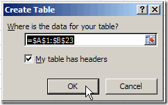
  • In the Create Table dialog box, the range for your data should automatically appear, and the My table has headers option is checked. Click OK to accept these settings.
  • CreateTableOK

Explore the Excel Table Features

After you have created an Excel Table, you can test some of its useful features:

  • Sort Data — Click drop down arrow in the heading cells, and click to sort data in ascending or descending order.
  • Quick Filters — Click drop down arrow in the heading cells, and check or uncheck items to show or hide.
  • Visible Headings – If headings in row 1 are no longer visible, column letters are replaced by Excel Table headings.
  • New data automatically included–Add data at the end of an Excel table, and the table automatically expands to include it.
  • Table Name –An Excel table is automatically named, e.g. Table1, when it is created. You can refer to this name when creating a pivot table. You can also change the name to something better, such as SalesData.

Excel Table Tutorial Video

If you’re working with lists of data in Excel 2007, be sure to use the new Excel Table feature, to make it easier to manage your data.

To see a quick demonstration of creating an Excel Table, and testing a few features, please watch this short video tutorial.

____________
Rename a Pivot Table Data Field

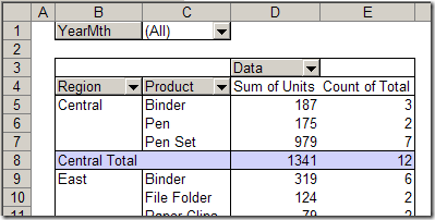
When you add a field to the pivot table Data area, it automatically gets a custom name, such as Sum of Units or Count of Units. You can rename a pivot table data field, either manually or with a macro.

PivotDataNames01

Instead of “Sum of Units”, you might want the name to show as “Units”, so it’s easier to read and the column is narrower.

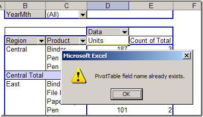
Unfortunately, if you select the cell and type Units, you’ll see an error message: “PivotTable field name already exists.”

rename a pivot table data field

When you try to use a custom name that’s identical to a field name in the source data, you’ll see that error message. In this example, one of the fields in the source data is named Units, so you can’t use Units as a custom name in the pivot table.

Use a Slightly Different Custom Name

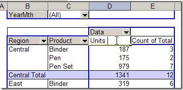
To avoid this problem, you can add a space character to the end of the custom name, and it will be accepted.

In the screen shot below, I’ve added a space after typing Units. When I press the Enter key, the name will be accepted, without an error message.

PivotDataNames03

Use a Macro to Rename a Pivot Table Data Field

If you have lots of Data field names to change you could use a macro, to make the job easier. For example, the following macro will change all the Data field captions in the first pivot table on the active sheet.

Sub ChangeCaptions()
Dim pf As PivotField
Dim pt As PivotTable
Set pt = ActiveSheet.PivotTables(1)
For Each pf In pt.DataFields
    pf.Caption = pf.SourceName & " "
Next pf
End Sub

There are instructions here for adding code to your workbook, and running it. This code would go onto a regular module.

There are more code samples on my Contextures website, for changing headings in:

  • all pivot tables on the active worksheet
  • all pivot tables in the active workbook.

___________________________

Copy a Custom PivotTable Style

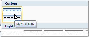
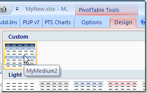
You can create custom PivotTable Styles in an Excel 2007 workbook, to fine tune the appearance of your pivot tables. If you’ve invested a lot of time in create a custom style, you might like to copy that style to a different workbook.

PivotCustomStyleMed

Unfortunately, there isn’t a built-in command that will let you copy PivotTable Styles from one workbook to another. However, you can follow a few simple steps to copy your styles to any workbook.

Copy a PivotTable Style

To copy a custom PivotTable style, you can temporarily copy a formatted pivot table to a different workbook. In this example, we’ll copy a custom PivotTable Style – MyMedium2 – from the MyOld.xlsx workbook to the MyNew.xlsx workbook.

  1. In the MyOld.xlsx workbook, select a cell in the pivot table that has the custom style applied.
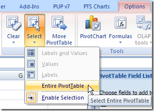
  2. On the Ribbon’s Options tab, in the Actions group, click Select.PivotTableSelect
  3. Click the Entire Pivot Table command.
  4. On the Ribbon’s Home tab, click Copy.
  5. Switch to the MyNew.xlsx workbook.
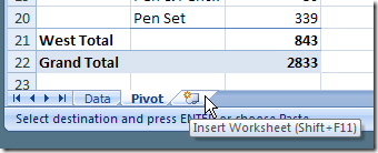
  6. Select a blank worksheet, or insert a new blank worksheet.SheetInsert
  7. Select cell A1 on the blank worksheet.
  8. On the Ribbon’s Home tab, click Paste.
  9. Delete the sheet that contains the pasted copy of the pivot table.

Your custom PivotTable style now appears in the PivotTable Styles gallery.

PivotCustomStyle

Select any pivot table in the workbook, and apply your custom PivotTable Style.

Watch the Video

_____________________

For more information on Pivot Tables, please visit Pivot Table Topics index on the Contextures Website.

_____________________