Quickly Add Fields in Excel 2003 Pivot Table

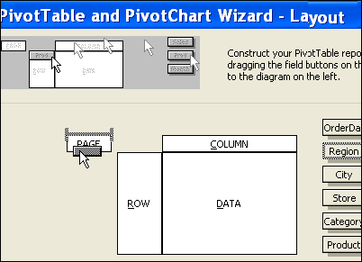
When you have a long list of fields in an Excel 2003 pivot table, it can take a long time to drag them into the pivot table layout, using the PivotTable Wizard.

pivotfieldadd00

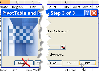
For a quicker way to add the fields, don’t go into the Layout screen in Step 3 — just click the Finish button.

pivotfieldadd01

Add Fields from the PivotTable Field List

When the PivotTable Wizard closes, you’ll see a blank pivot table on the worksheet.

Note: If the PivotTable Field List isn’t visible, click the Show Field List button on the PivotTable Toolbar.

pivottoolbarshowfieldlist

To add the pivot fields:
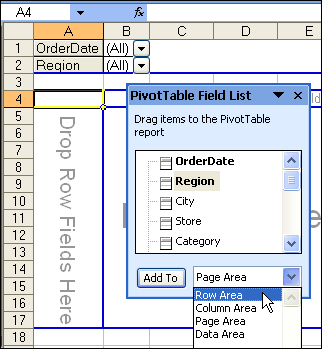
  1. Then, in the Field List, select one of the layout areas from the drop down list.
    • pivotfieldadd02
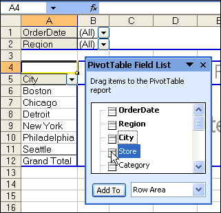
  2. In the Field List, double-click on each field that you want to add to the selected layout area.
    • pivotfieldadd03

Repeat Steps 1 and 2, for all the layout areas, leaving the Data Area to fill in last.

____________

Use Pivot Table Calculated Item

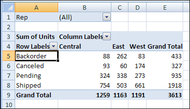
If you need to sum specific items in a pivot table field, you can create a calculated item. For example, if your pivot table contains an Order Status field, with four types of status:

  • Shipped
  • Pending
  • Backorder
  • Canceled

You could create a calculated item, named Sold, that sums the units sold, for orders with a status of Shipped, Pending, or Backorder.

Create a Calculated Item

Follow these steps to create a calculated item:

  1. In the pivot table, select a cell that contains an Order Status item. For example, select cell A5, that contains the Backorder item.calculateditem01
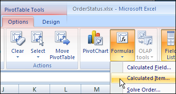
  2. On the Ribbon’s Options tab, in the Tools group, click Formulas, and then click Calculated Item.calculateditem02
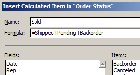
  3. Type a name for the Calculated Item, for example, Sold, and then press the Tab key to move to the Formula box.
  4. In the Fields list, select Order Status, and in the Items list, double-click Shipped, and then type a plus sign (+).
  5. Double-click Pending, type a plus sign, and then double-click Backorder. The complete formula is =Shipped+Pending+Backorder.calculateditem03
  6. Click OK, to save the calculated item, and to close the dialog box.

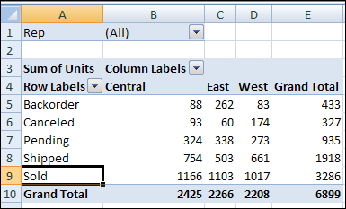
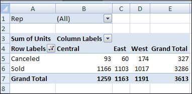
The new calculated item, Sold, is added to the Row area in the pivot table. However, the Grand Totals have increased, because the Sold item includes the values from other items.

calculateditem04

Hide the Unnecessary Pivot Items

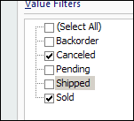
In the pivot table, you can hide the Shipped, Pending, and Backorder items, because they are included in the Sold calculated item.

calculateditem05

With those pivot items hidden, the pivot table will show the correct Grand Totals.

calculateditem06

Download the Sample File

To see the pivot table data and the calculated item, you can download the sample file from the calculated item page on my Contextures website.

In the Download section, click on the first item — Create a Calculated Item sample file.

The file is in xlsx format, and is zipped.

_______________

Highlight Pivot Filters With Markers

One of the benefits of using an Excel pivot table to analyze your data, is that you can use filters to focus on a specific part of the summarized results. Hiding some of the data with filters can be misleading though, if you can’t tell that filters have been applied.

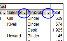
If you apply a filter in Excel 2007 or Excel 2010, the filter drop down changes to a funnel, with a tiny arrow. In the screen shot below, the ItemSold field has been filtered, to hide some of the items.

pivotfiltermarkers00

In Excel 2003, and earlier versions, if you apply a filter to a pivot field, the drop down arrow doesn’t change. The same filter was applied in Excel 2003, in the screenshot below, but both drop down arrows are the same.

pivotfiltermarkers02

Create Your Own Filter Markers

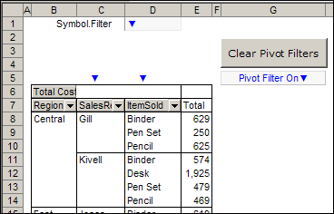
If you’d like to make it easier to tell which fields are filtered, you can use the Excel VBA code created by AlexJ, which displays a bright blue marker above each filtered field.

pivotfiltermarkers

Download the Sample File

To test the pivot table filter markers, and see the VBA code, you can download AlexJ’s sample file from the Contextures website. On the AlexJ Sample Files page, go to the Pivot Tables section, and look for:  PT0000 – Pivot Table Filter Markers

__________


Copy Pivot Table Values and Formats

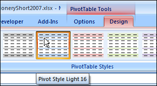
If you create a pivot table in Excel 2007 and later versions, formatting is automatically applied by the PivotTable Styles feature.

PivotStyles01

This feature makes it quick and easy to format your pivot tables, and helps you stay consistent with the Theme settings in your Excel file.

Problems with Format Copying

Occasionally, you might want to copy a pivot table as values, without the underlying data. Unfortunately, if you copy an Excel 2007 or later pivot table, and paste it with the Paste Special command, the PivotStyle formatting is not pasted.

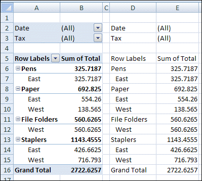
In the screenshot below, the values from the pivot table were pasted into columns D:E, but pasting the formats had no effect.

pivotcopyformat

Pivot Table Format Paste Workarounds

Fortunately, there are workarounds for the problem of pasting the pivot table formatting:

  1. Use the Office Clipboard, to paste the Pivot Table formatting
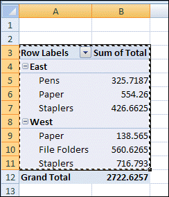
  2. Copy and paste the pivot table in a couple of steps, as shown below
  3. Programmatically copy the pivot table in a couple of steps

pivotbodycopy02 

___________

Problems With Pivot Table Comments

In some pivot tables, you might want to add comments to a few cells, to help the users understand what the results mean, or to explain the different pivot fields. However, if you add comments to a pivot table, you’ll run into a couple of problems.

Add a Comment to the Pivot Table

The Insert Comment command doesn’t appear in the popup menu if you right-click on a pivot table cell.

To insert a comment in a pivot table:

  1. Select the cell where you want the comment.
  2. On the Excel Ribbon, click the Review tab
  3. Click New Comment

Tooltips Block the Comments

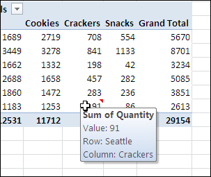
One problem with comments in a pivot table is that the contextual tooltips might appear when you point to a pivot table cell that contains a comment. In the screen shot below, you can see the red comment marker, but the comment isn’t visible.
Comments01

If you decide to use comments, follow these steps, to turn off the tooltips feature.

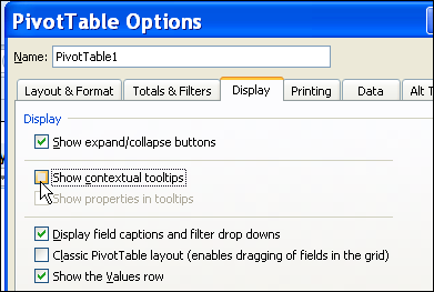
  1. Right-click a cell in the pivot table, and then click PivotTable options.
  2. In the PivotTable Options dialog box, on the Display tab, remove the check mark from Show contextual tooltips and then click OK.
Comments02

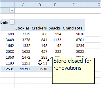
After you turn off this setting, the comment appears when you point to the cell.
Comments03

Pivot Table Comments Don’t Move

When you add comments to cells in the pivot table, the comments are attached to the Excel worksheet cell, rather than to the pivot item’s cell. If you change the pivot table layout, the comments won’t move with the item, and the comments could end up confusing the users instead of helping them.

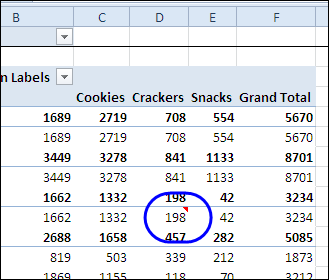
In the screen shot below, a new field has been added to the row area. The comment was originally added to cell D10, that had a value of 91, for cracker sales in Seattle. Now the layout has changed, but the comment is still in cell D10. That cell now has a value of 198, and summarizes cracker sales at store 3074 in Detroit.
Comments04

Alternative to Comments

Instead of inserting comments in the pivot table, you could add a column to the source data, and enter brief comments there. A user who has a question about the data in the pivot table could double-click on the cell, using the Show Details feature to extract the source data and read any notes entered.

___________
Locate Pivot Table Source Access File And Query

For a pivot table that’s based on a Microsoft Access query, you might need to find out which database and query were used as the source data.

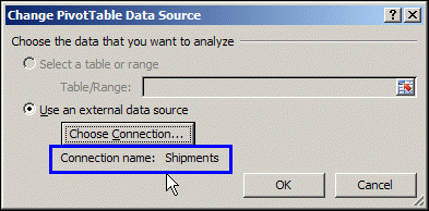
In Excel, if you click the Change Data Source command, on the Ribbon’s Options tab, you can see the connection name in the Change PivotTable Data Source dialog box. However, that bit of information isn’t too useful — it doesn’t show you the name and path of the Access file, and you can’t see which query was used to create the pivot table.

sourcequery01 

View the Connection Properties

To find the details on the source data’s Access file and query, you can follow these steps:

  • In the Excel file, select a cell in the pivot table
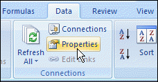
  • On the Ribbon’s Data tab, in the Connections group, click Properties.

ribbondataproperties

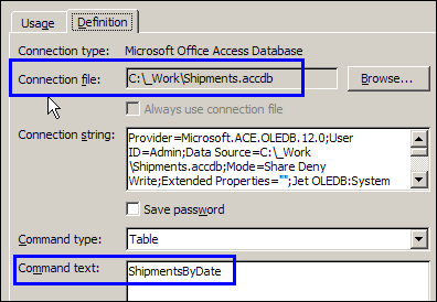
  • In the Connection Properties dialog box, click the Definition tab.
    • In the Connection File box, you can see the name and path of the database.
    • In the Command Text box is the name of the Access query.
  • Click Cancel to close the Connection Properties dialog box.

sourcequery02

______________

Apply Multiple Filters to Pivot Table Field

A powerful feature of pivot tables is that you can filter a pivot field, to see specific results. However, if you apply a different filter to that pivot field, the first filter is removed. For example, if you filter a Row field for region names starting with “East”, and then add a Top 10 filter, the “East” filter is removed.

Use the technique shown in this video to apply multiple pivot table filters at the same time. You can use a Label filter, Value filter and Manual filter simultaneously, to fine tune your pivot table reports.

__________

Special Price Today on Microsoft PowerPivot Ebook

If you’re interested in learning how to use Microsoft PowerPivot for Excel 2010, here is a bargain for you.

There’s a special price today on the ebook version of Microsoft PowerPivot for Excel 2010: Give Your Data Meaning, by Mark Russo and Alberto Ferrari.

Here’s the tweet that announced the special price:

#Ebook Deal of the Day: Microsoft PowerPivot for Excel 2010 – $14.99 (Save 46%) Code DDPVT

The link in that tweet takes you to the O’Reilly page, where it shows the full price. Just click the “Add to Cart” button for the Ebook version, and enter the special code (DDPVT).

Newer Version

Update: There is a newer version of this book available now — Microsoft Excel 2013 Building Data Models with PowerPivot

___________

PowerPivot Contest

powerpivoticon If you love the new PowerPivot add-in for Excel 2010, you can enter the latest contest on the PowerPivotPro blog. Show off your efficient PowerPivot techniques, and win one of the two top prizes — a 1 year MSDN subscription.

Send in your sample workbooks, with charts and slicers and cross-filtering enabled. Impress Rob with your PowerPivot skills, and you might win one of the top prizes, or a PowerPivot poster.

Here’s how Rob will decide the winner:

Entries will be judged on, in roughly descending order:

  1. Performance – I will compare query speed with slicer cross-filtering turned on vs. turned off.  Smaller differences are better for this contest.
  2. Polish – as I slice the report, do the charts all still look nice?  Ex:  Blank space in charts = not good.
  3. Ease – how hard is it to execute your technique?  We will turn winning entries into blog posts, and this will become a new reference technique here at PowerPivotPro.
  4. Originality – this never hurts but is not crucial.  Fun is good.  Unexpected benefits and features are even better.

I don’t see a closing date for the contest, so you’d better get started soon, and send in your entry ASAP.

Update: Contest closes Sunday October 3rd, 11:59 PM US Pacific time

dashboardsheet_thumb

___________

Improve Performance When Changing Pivot Table Layout

If your pivot table is based on a large data source, it might respond very slowly when you add fields or move fields to a different area of the pivot table.

To improve performance, try the following tips:

  • Remove any pivot table styles and any other formatting, such as conditional formatting that you applied to the pivot table.
  • Calculated items can negatively impact the speed of updating. If possible, remove any fields that contain calculated items, or delete the calculated items from the fields.

Defer Layout Update

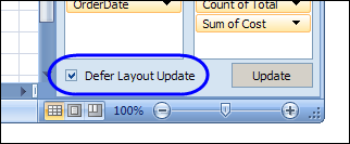
If you plan to add or move more than one field, you can use the Defer Layout Update option. When this feature is enabled, the fields are all added or moved, and then the pivot table is recalculated once. If this box is not checked, the pivot table is recalculated after each field is added or moved.

To defer the layout updates:

  • Add a check mark to the Defer Layout Update box in the PivotTable Field List.

deferlayout

  • Move or all all the fields that you want to adjust
  • Click the Update button, to the right of the Defer Layout Update check box.
  • When you’re finished changing the layout, remove the check mark from the Defer Layout Update check box.

Note: Some features, such as filtering and grouping, are not available when Defer Layout Update is activated.

_____________