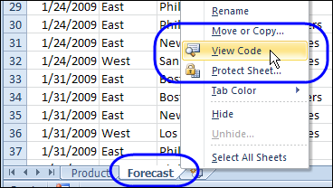
One of the most useful new tools in Excel 2010 is the Excel Slicer. Add a Slicer to the workbook, and you can filter multiple pivot tables with a single click. Here is a warning for Excel 2010 Slicers though, and if you use the Drill to Details feature
Unique Count in Pivot Table With Excel PowerPivot
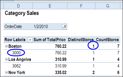
In Excel 2010, there is no built-in summary function that calculates a distinct count or unique count in a pivot table. In the pivot table shown below, we’d like to see the number of stores in Boston, where each product category was sold.
Continue reading “Unique Count in Pivot Table With Excel PowerPivot”
Sorting Pivot Table Report Fields
To focus on specific data in an Excel pivot table, you can add a field to the Report Filter area. Then, select one or more items from that pivot table field, to see the summarized data.
If you put a date field in the Report Filter area, there might be a long list of dates in the dropdown list. When you create the pivot table, the dates are usually in ascending order, with the oldest dates at the top of the list.
That’s not too convenient, if you want to focus on the latest data, instead of the oldest. How can you change the sort order, to put the newest dates at the top of the list?
Sort the Report Filter Field
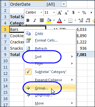
Usually, it’s easy to sort a pivot table field. For example, if you right-click on a field in the Row area, the popup menu shows sorting and grouping options.
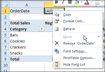
However, when you right-click a Report Filter field, those sorting and grouping options aren’t listed in the popup menu.
Move the Pivot Table Field
To solve the sorting problem, you can use a workaround – temporarily move the Report Filter field to the Row Labels area.
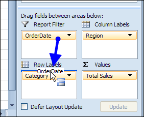
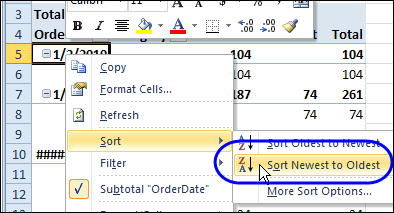
Then, use the right-click popup menu to sort the date field in descending order.
Drag the field back to the Report Filter area, after you sort it.
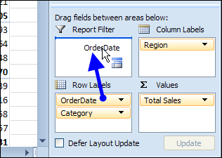
Report Filter Dates in Descending Order
After you sort the field in descending order, you’ll see the latest dates at the top of the drop down list.
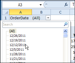
It’s not the ideal solution, but it works! Maybe in the next version of Excel you’ll be able to sort the fields, without moving them from the Report Filter area.
Video: Sort Report Filter Field
Watch this very short video, to see how to show the items alphabetically, by temporarily moving the Report Filter field to the Rows area in the pivot table.
Download the Sample File
To download the sample file, please visit the Pivot Table Sorting page on my Contextures website.
_________
Repeat Pivot Table Labels in Excel 2010
When you create a pivot table in Excel 2010 or Excel 2007, the row labels are in a compact layout – all the headings are listed in column A.
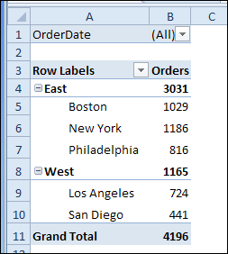
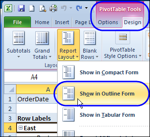
You can change the Report Layout setting, to either Outline form or Tabular form, so each row field is in a separate column.
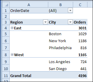
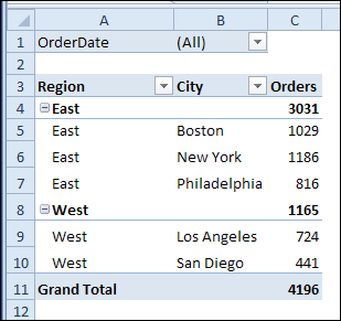
Here’s the same pivot table in Outline form. The Region field is in column A, with a separate row for each new heading.
Repeat the Row Labels
A new feature in Excel 2010 lets you repeat those row labels, so they appear on every row in the pivot table.
To turn on that feature for all the fields, select the Repeat All Item Labels on the Ribbon’s Design tab.
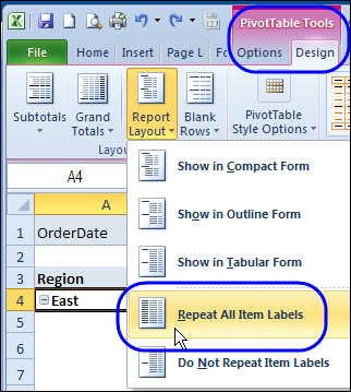
Here’s the pivot table in Outline form, with repeating row labels.
Repeating Labels for a Single Field
Instead of turning on repeating labels for the entire pivot table, you can apply the feature to a specific pivot table field.
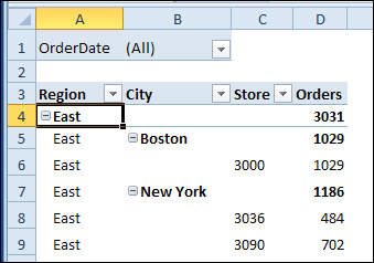
In this example, the Region, City and Store fields are in the Row area, and we’ll turn on repeating labels for the Region field only.
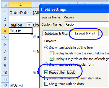
- Right-click one of the Region labels, and click Field Settings
- In the Field Settings dialog box, click the Layout & Print tab
- Add a check mark to Repeat item labels, then click OK
Now, the Region labels are repeated, but the City labels are only listed once.
Watch the Pivot Table Repeat Labels Video
To see the steps for repeating labels in all fields, or a single field, please watch this short Excel pivot table video tutorial.
_________________
Student Budget With Pivot Tables: Spreadsheet Day 2011
 Happy Spreadsheet Day! We celebrate on October 17th, because this is the date that VisiCalc was first released to customers, in 1979. This year’s theme is Spreadsheets for Students, and what better way to help students, than show them a great way to use pivot tables?
Student Budget Workbook
Most students have limited funds, so it’s important that they plan and track their spending. Bob Ryan, from the Simply Learning Excel website, has created a Student Budget spreadsheet, that should help students get their finances organized.
There is a transaction sheet, where you can enter your budget amounts and track your actual spending, including cash and credit cards. At the end of the month, review your cash and credit card spending in pivot tables that shows monthly totals.
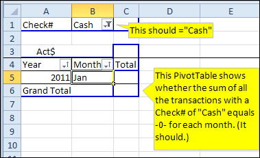
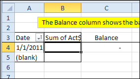
In another pivot table, you can keep track of your running balance.
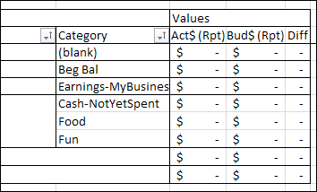
Bob also built a pivot table which compares your budget amounts with the actual amounts.
Download the Student Budget Workbook
You can download the Student Budget Spreadsheet file, and use it to track your own finances. To get the file, go to the Excel Sample Files page on my Contextures website, and in the Pivot Tables section, look for PT0023A – Student Budget Workbook. The file is in xlsx format, and it is zipped. There are no macros in the file.
Contribute to Spreadsheet Day 2011
If you’d like to join the Spreadsheet Day celebrations, please post your own free and useful spreadsheet template or add-in, that will help students get organized. Or, if you prefer, post a tip or link in Twitter, with the hashtag #spreadsheetday
Thanks for joining the Spreadsheet Day celebrations, and for sharing your knowledge with students. I’m sure they’ll appreciate it!
___________
Excel Pivot Table: Refresh Automatically With Macros
When you update a pivot table’s source data in Excel, the pivot table does not update automatically. You can set the pivot table to update when the Excel file opens, but that doesn’t help if you’re making changes after the file opens. If you can use macros in your Excel file, you can use an event procedure to force the pivot table to refresh automatically if the source data changes.
Continue reading “Excel Pivot Table: Refresh Automatically With Macros”
Check for Shared Pivot Cache
Last year, I posted Excel VBA code for removing a calculated field from a pivot table.
The code works well if there is only one pivot table based on that pivot cache. However, a couple of comments mentioned that there were problems if multiple pivot tables shared the pivot cache.
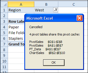
Here is a revised version of the code, that checks for other pivot tables using the same pivot cache. If others are found, the macro is cancelled, and a message appears, listing the pivot tables.
Remove Calculated Fields for Non-Shared Pivot Cache
If other pivot tables in the workbook share the same cache, the macro is cancelled. A message lists those pivot tables.
Sub RemoveCalculatedFieldsNotShared()
Dim ws As Worksheet
Dim ptA As PivotTable
Dim pt As PivotTable
Dim pf As PivotField
Dim pfNew As PivotField
Dim strSource As String
Dim strFormula As String
Dim iPC As Long
Dim lCache As Long
Dim strPC As String


Set ptA = ActiveSheet.PivotTables(1)
iPC = ptA.PivotCache.Index

For Each ws In ActiveWorkbook.Worksheets
    For Each pt In ws.PivotTables
        If pt.PivotCache.Index = iPC Then
            lCache = lCache + 1
            strPC = strPC & ws.Name & "     " _
                & pt.TableRange2.Address _
                & vbCrLf
        End If
    Next pt
Next ws

If lCache > 1 Then
    MsgBox "Cancelled" _
        & vbCrLf & vbCrLf _
        & lCache & " pivot tables share this pivot cache: " _
        & vbCrLf & vbCrLf _
        & strPC
    GoTo exitHandler
Else
    For Each pf In ptA.CalculatedFields
        strSource = pf.SourceName
        strFormula = pf.Formula
        pf.Delete
        Set pfNew = ptA.CalculatedFields.Add(strSource, strFormula)
    Next pf
End If

exitHandler:
    Exit Sub

End Sub
_______________
Quickly Remove Pivot Table Grand Totals
You probably know how easy it is to add or remove the Grand Totals in a pivot table, by using the Ribbon commands.
But keep reading, to see an even quicker way!
Grand Totals on the Ribbon
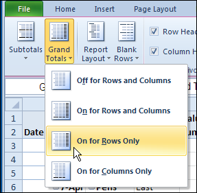
Yes, it’s easy to change the Grand Total settings on the Ribbon:
- Select any cell in the pivot table
- On the Ribbon, under PivotTable Tools, click the Design tab
- In the Layout group, at the left, click Grand Totals
- Click one of the options.
Quickly Remove Grand Totals
For an even quicker way to remove Grand Totals, follow these steps:
- In the pivot table, right-click the Grand Total label cell (not the total amounts) – either the Row Grand Total or the Column Grand Total
- In the popup menu, click Remove Grand Total
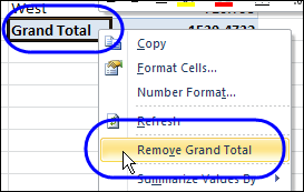
That’s it! Unfortunately, there’s no equally quick way to add Grand Totals, but maybe that feature will be in the next version of Excel.
________
Excel Pivot Table for Financial Data
Last week, you saw a technique for changing monthly data into a better layout, when creating an Excel pivot table.
We used a multiple consolidation ranges pivot table to change this 13-column table into a 3-column data source.
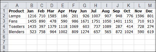
Today we’ll look at a different approach to using multi-column data in a pivot table.
Bi-Weekly Data
Thanks to Jim LaBarr, who sent me a sample Excel file, with his solution to creating reports from multi-column financial data.
In his file, Jim has dates in the heading row – not just the month names. Every column has a heading, and there are no blank rows or columns within the data.
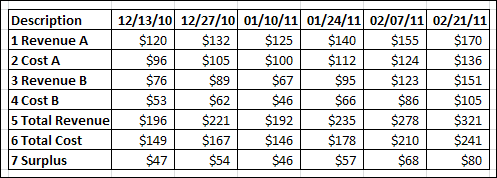
NOTE: Usually, Jim would create an Excel Table from this data, but that changes the headings to text. Don’t create an Excel Table if you want to use the technique that Jim is sharing today.
Pivot Table from Bi-Weekly Data
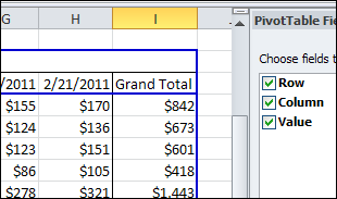
After setting up his bi-weekly financial data, Jim creates a pivot table, using multiple consolidation ranges. This creates a pivot table with 3 fields – Row, Column and Value.
The dates are the Column items, and the descriptions are the Row items.
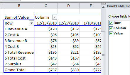
This multiple consolidation ranges pivot table shows a grand total for the columns, because all the dates are in the Column field.
NOTE: If we had created a normal pivot table from the data, each date would be a separate field, and there would be no grand total.
Filter the Pivot Table
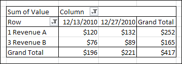
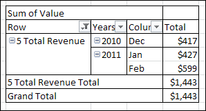
After creating the pivot table, Jim filters the Row and Column fields, to focus on specific data. For example, you could filter the Rows to show only the Revenue items (but not the Revenue Total). Then, filter the Columns, to show the December 2010 dates.
The Row and Column grand totals automatically update, to show the totals for the filtered pivot table.
Change the Pivot Table Values
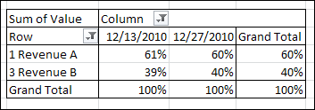
When you create a pivot table, the values are summarized by Sum or Count, and shown as simple totals. For a different view of the data, Jim changes the way the Values are shown. In the pivot table shown below, the Values are shown as % of Column.
This is a quick way to see the revenue breakdown, for the two revenue streams. Revenue A produces 60% of the revenue, and 40% is from Revenue B.
Grouping the Dates
Because the multiple consolidation ranges pivot table puts the Dates in a single field, Jim is able to group those dates. This gives him even more flexibility in his pivot table reports.
Here, the dates are grouped by year and month, and again, the grand totals are automatically calculated.
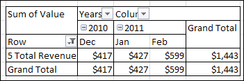
Or, the Column field can be moved to the Row area, to show the dates at the left, in a vertical report.
Additional Summary Functions
In another version of his pivot table report, Jim puts 3 copies of the Value field in the Values area.
- Sum
- Change
- % Change
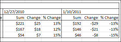
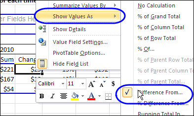
To show the Change, Jim changes the custom calculation to Difference From. For % Change, Jim uses the % Difference From custom calculation.
Create a Pivot Chart
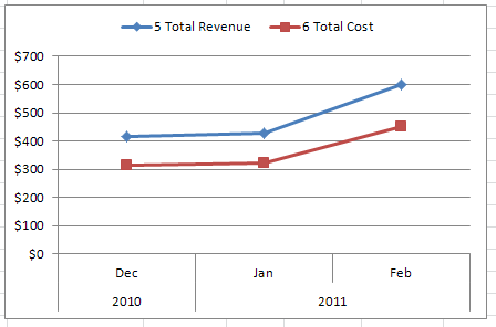
To give a visual overview of the data, Jim create a pivot chart from the multiple consolidation range pivot table. Here, the Years and Months are in the Row area, and the Descriptions are in the Column area, filtered for Total Cost and Total Revenue.
Jim’s Tips for Financial Data Pivot Tables
If your financial data is in many columns, like Jim’s example, here are Jim’s tips for when to use this multiple consolidation ranges techniques, and when to use an Excel Table instead.
- Use this method to keep multiple columns, with pivot table benefits, like date grouping
- Use Tables if all you need is Filtering on Rows
- Use Tables if you need Chart of multiple Rows with no need for time period Grouping
- For source data with multiple description columns, use the normalization workaround
Download the Sample Financial Data Pivot Table File
To see Jim LaBarr’s sample data, and the pivot tables, you can download his Financial Data Pivot Table sample file. The file is in Excel 2003 format, and zipped.
______________
Friday Fun: Pivot Table Comic
It’s Friday, and the weather has been unbearably hot all week. On top of that, your boss and/or Excel are making you crazy.
If you’re on your last nerve, you can vent your rage in a comic strip, by using Rage Builder. I made this pivot table themed comic, and I’m sure you can do better!
I didn’t upload my comic to the website – I used Snagit to take a screen shot, and save that image file.

________

