Refresh Pivot Table on Protected Sheet

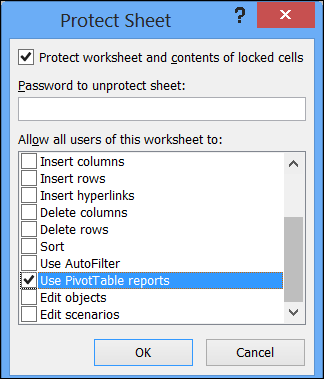
When you protect a worksheet in Excel, you’ll see a list of items that you can allow people to use, while the sheet is protected.

One of those options is ‘Use PivotTable reports’, and if you add a check mark to that option, things might not work exactly as you expected.
refreshpivotprotectedsheet03

Limited Use of Pivot Tables

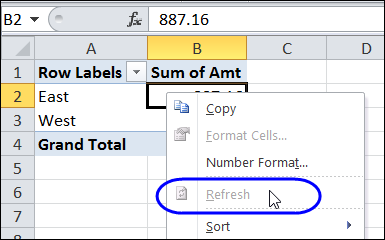
When the sheet is protected, even if you have allowed pivot table use, you can’t create a new pivot table. Another restriction is that you won’t be able to refresh a pivot table on the worksheet. If you right-click in a pivot table cell, the Refresh command is disabled.
refreshpivotprotectedsheet02

Refresh on Protected Sheet

If you need to refresh a pivot table on a protected sheet, you could

  • manually unprotect the worksheet
  • refresh the pivot table
  • protect the sheet again

Another option, if you would prefer to refresh the pivot table programmatically, is to create a macro that does these steps for you. The following macro will refresh the first pivot table on the active sheet, which has a password – “mypassword”

Sub UnprotectRefresh()
On Error Resume Next

With Activesheet
  .Unprotect Password:="mypassword"
  .PivotTables(1).RefreshTable
  .Protect Password:="mypassword"
End With

End Sub

Connected Pivot Tables

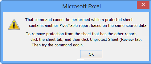
If other pivot tables are connected to the same pivot cache are on protected sheets, you won’t be able to refresh a pivot table, even if it is on an unprotected sheet.
refreshpivotprotectedsheet01

In this situation you will have to unprotect the sheet(s) where those other pivot tables are located, and then do the refresh.

There is sample code to unprotect all the sheets, and do a refresh all, on my Contextures website: Refresh Pivot Table Connected to Protected Sheet

_______________________

Show Value Weight With Pivot Table Index

You might have used one of the Custom Calculations in a pivot table, such as % of Column or Running Total. There’s another Custom Calculation – Index — that isn’t used very often, but provides an interesting look at the pivot table values.

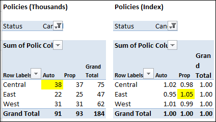
In the screen shot below you can see the original data in the pivot table, and the same date using the Index custom calculation. Even though Central Auto is the highest value in the table at the left, East Property has the highest Index value.

customcalculationindex01

Using the Index custom calculation gives you a picture of each value’s importance in its row and column context.

  • If all values in the pivot table were equal, each value would have an index of 1.
  • If an index is less than 1, it’s of less importance in its row and column
  • If an index is greater than 1, it’s of greater importance in its row and column.

The Index Formula

Even if two cells have the same value, they may have a different index. The Index formula is:

customcalculationindex05

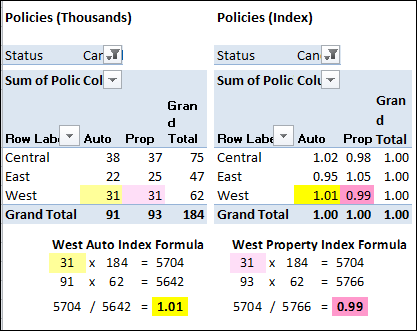
So, in this example, in the West region, the values for Auto and Property are almost equal, but the index for the Auto is 1.02 and Property is 0.98.

Because the grand total is higher for the Property column, the Grand Column Total in the Index formula is larger. The West Property amount is divided by this larger number, and its resulting index is smaller.

customcalculationindex06

Read more about Index and the other Pivot Table Custom Calculations on my Contextures website.

______________________

Hide Drop Down Arrows in Pivot Table Headings

When you add a field to the Row Label or Column Label area of the pivot table, its heading cell shows a drop down arrow. When you click the arrow, you’ll see Sort and Filter options, for the selected field.

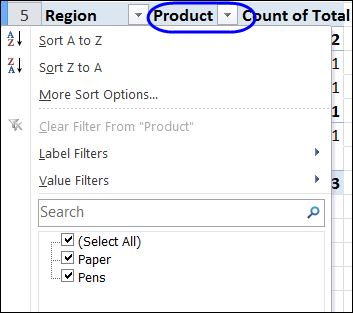
In the screen shot below, you can see the sort and filter options for the Product field, and the check boxes for manually filtering the list.

labelfilter01

Hide the Arrows

If you want to prevent manual filtering, you can hide the drop down arrows, by using a bit of Excel VBA programming.

The following code will hide the drop down arrow for every field in the first pivot table on the active worksheet.

Sub DisableSelection()
Dim pt As PivotTable
Dim pf As PivotField
Set pt = ActiveSheet.PivotTables(1)
  For Each pf In pt.PivotFields
      pf.EnableItemSelection = False
  Next
End Sub

Sorting and Filtering Still Available

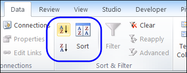
After you hide the arrows, you will still be able to sort the pivot items, by using the commands on the Ribbon.

ribbonsort01

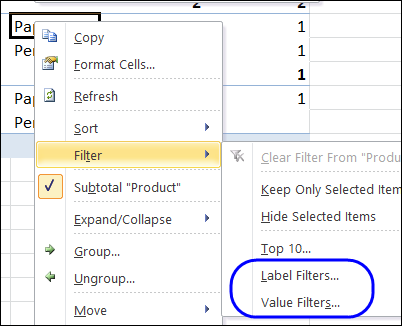
You’ll also be able to use the Label Filters and Value Filters, if you right-click on an item in the disabled field.

labelfilter02

Show the Arrows

After you hide the arrows, you can use similar code to show them again — just change the EnableItemSelection setting to True.
The following code will show the drop down arrow for every field in the first pivot table on the active worksheet.

Sub EnableSelection()
Dim pt As PivotTable
Dim pf As PivotField
Set pt = ActiveSheet.PivotTables(1)
  For Each pf In pt.PivotFields
      pf.EnableItemSelection = True
  Next
End Sub

Video: Apply Multiple Filters to Pivot Field

To see the different types of filters – label, value and manual – please watch this short video tutorial.

Or watch on YouTube: Apply Multiple Filters to Pivot Table Field

________________

Create Custom Ribbon Tabs for Workbooks

If you’re creating workbooks with pivot table reports, you might have macros in those files, to make it easier to work with the pivot tables, or to navigate through the workbook sheets.

Instead of creating buttons on the worksheets, to run the macros, you can create a custom tab on the Excel Ribbon, with buttons to run the macros.

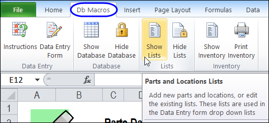
For example, this sample file lets users enter parts data in a UserForm, and summarizes the current inventory in a pivot table. The “Db Macros” tab appears when this workbook is active, and disappears when it’s not active.

ribbonpartdb01b

Getting Started with Custom Ribbon Tabs

In the following video, you can see how to view the code for a custom Ribbon tab, and make a minor change. The written instructions are on my Contextures website, where you can also download the sample file: Excel Ribbon – Getting Started.

Create Your Own Custom Ribbon Tab

In the next video, you’ll see how to start from scratch – add a custom tab, create the code, and modify it. Then, make a slight change to the macros in Excel, and the Ribbon buttons will run your macros. The written instructions are on my Contextures website, where you can also download the sample file: Excel Ribbon – Add a Custom Tab.

_________________

Number of Records in Pivot Table Source

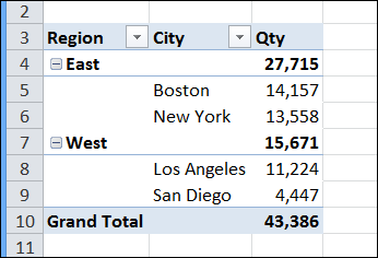
When you create a pivot table, it is based on a pivot cache, with all of the records from the source data table. You can’t see the pivot cache, but with some programming, you can get information about the cache.

pivotcacherecordcount01

In the pivot table shown above, you can see the total quantities for all the records in the source data. To see how many records are in that source data, you can create a User Defined Function.

Create a User Defined Function

To create the User Defined Function, copy the following code, and paste it into a regular code module.

Function GetRecords(rngPT As Range) As Long
'pivot table tutorial by contextures.com
  Dim pt As PivotTable
  Set pt = rngPT.PivotTable
  GetRecords = ActiveWorkbook _
    .PivotCaches(pt.CacheIndex).RecordCount
End Function

This creates a function named GetRecords, and it requires a cell reference as its argument. If the referenced cell is in a pivot table, the function will show the record count for that pivot table’s pivot cache.

Note: If you save this file, make it a macro-enabled file type.

User a User Defined Function

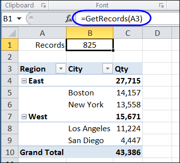
Then, on a worksheet in that workbook, enter a formula that uses the function name, and refers to a cell in the pivot table. For example, enter the following formula in cell B1, referring to the pivot table in cell A3:

=GetRecords(A3)

pivotcacherecordcount02

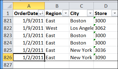
The formula result is 825, which is the number of records in the source data. You can see the last record in the screen shot below. It’s in row 826, and if you subtract 1 for the heading row, that is record number 825.

pivotcacherecordcount03

______________

Use Dates in GetPivotData Formula

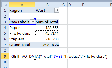
With a GetPivotData formula, you can pull data from a pivot table. For example, how many file folders were sold:

getpivotdata02

The formula works well with text fields, but you might get errors if you create a formula using dates.

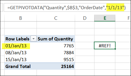
In the example shown below, the formula in cell E4 refers to the date “1/1/13”, but the result is a #REF! error, even though that date is in the pivot table.

=GETPIVOTDATA(“Quantity”,$B$3,”OrderDate”,”1/1/13″)

getpivotdatadates01

To get the correct results for dates, you can use one of the following methods:

  • Match the pivot table’s date format
  • Use the DATEVALUE function
  • Use the DATE function
  • Refer to a cell with a valid date

For written instructions, please visit the GetPivotData page on my Contextures website.

Watch the Video

To see the steps for using dates in a GetPivotData formula, please watch this short video tutorial.

____________________

Change Pivot Table Data Headings and Blanks

When you add fields to the value area in a pivot table, custom names are automatically created, such as Sum of Quantity or Count of Customer.

pivotlabels01

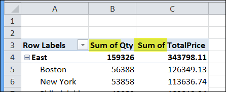
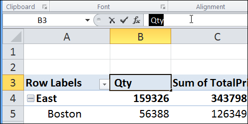
Excel won’t let you remove the “Sum of” in the label, and just leave the field name. However, you can change the heading to the field name, plus a space character, to work around this problem.

In the screen shot below, the heading has been changed to [space]Qty.

pivotlabels02

Change (Blank) Labels

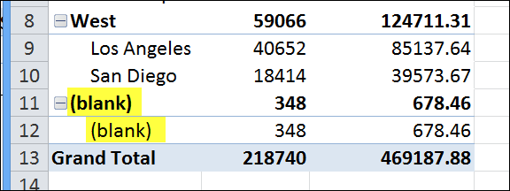
Another formatting fix that you can make is to get rid of the labels that say “(Blank”)”. These appear if cells are blank in the source data, and you add those fields to the row or column labels area.

pivotlabels03

Excel shows an error message if you just try to delete those labels, but you can use a space character to replace them.

Watch the Video

Watch this short video tutorial to see how to make these changes to the pivot table headings and labels.

________________________
Hide Calculated Items With Zero Total

In a pivot table, you can create calculated items, in addition to the pivot items from the source data. They can create problems in your pivot table layout, such as showing cities under every region, instead of just the region in which they’re located.

In this tutorial, I’ll create a calculated item in the Category field, and then fix the problem that it creates in the City field.

Pivot Table Setup

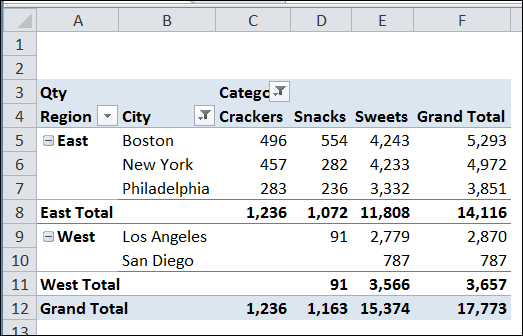
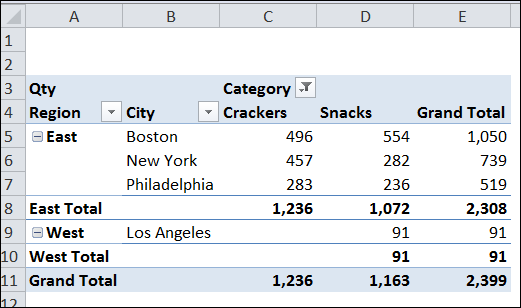
In the pivot table shown below, the Category field is in the Column headings, and it is filtered to show only two of the four categories – Crackers and Snacks.

The Region and City fields are in the Row headings, and there are 3 cities in the East and 2 cities in the West.

calcitemhidezero01

Create a Calculated Item

I want to add a new Category – Sweets – to show the total for the two hidden categories – Cookies and Bars.

To create the Calculated Item:

  • Select one of the Category heading cells, such as cell D4.
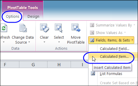
  • On the Ribbon, under PivotTable Tools, click the Options tab
  • In the Calculations group, click Fields, Items & Sets, and click Calculated Item

calcitemhidezero02

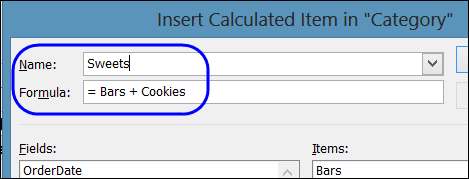
  • Type a name for the calculated item – Sweets
  • In the Formula box, enter the formula: =Bars + Cookies
  • Click OK, to Add the new item, and to close the Calculated Item window.

calcitemhidezero03

Calculated Item Problems

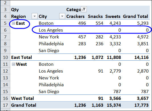
After you click OK, the Sweets category is added to the pivot table, in the Column Headings, as expected. However, each city is now listed under each region, with zero amounts in some rows.

calcitemhidezero04

What Went Wrong

When you add a calculated item, all the items are listed for fields that intersect the calculated item. The calculated item creates every possible combination of items in the intersecting fields, even if there is no data for that combination in the source data.

Unfortunately, you can’t change this behaviour – there’s no setting to turn it off. If possible, avoid calculated items, which can slow down a large pivot table, and create calculations in your source data instead.

Hide the Zero Rows

To hide the cities that are in the wrong region, you can use a pivot value filter to hide the rows with a zero total.

Note: This will also hide any other rows with zero grand total, so use this technique with caution.

  • Right-click a cell that contains a City row label, and in the context menu, click Filter, and then click Value Filters.
  • In the Value Filter window, from the first drop-down list, select Qty, which is the Values field you want to check.
  • In the second drop-down list, select does not equal
  • In the third box, type 0 (zero), and then click OK

calcitemhidezero05

The rows where the grand total is zero are hidden, and the wayward city names disappear from each region.

calcitemhidezero06

_____________________
Flexible Links to Pivot Table Data

To extract data from an Excel Pivot Table, you can use the GetPivotData function. Unless you change the default settings, a GetPivotData formula is automatically created if you type an equal sign, and then click on a pivot table data cell, to link to it.

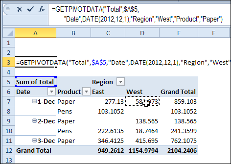
In the screen shot below, I typed an equal sign in cell A3, and then clicked on cell D7, which contains the total sales for:

  • Region: West
  • Product: Paper
  • Date: Dec 1st

The GetPivotData formula that was automatically created is:

=GETPIVOTDATA(“Total”,$A$5, “Date”,DATE(2012,12,1),”Region”,”West”,”Product”,”Paper”)

getpivotdata01

Replace Text with Cell References

Instead of leaving the text values in the formula, you can replace those values with cell references. This makes the formula flexible, and it will show a different result, based on the values in the linked cell.

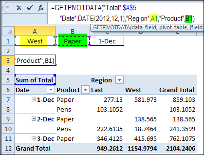
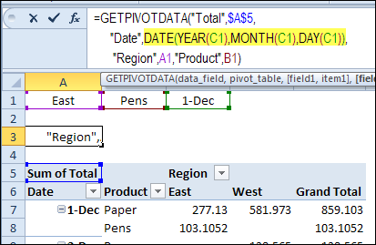
For example, I’ve entered a region name in cell A1, a product name in cell B1, and a date in cell C1.

Then, in the formula, I replaced “West” with a link to cell A1, and replaced “Paper” with a link to cell B1.

getpivotdata02

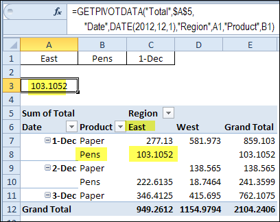
The formula result will now change automatically if I type East in cell A1, and type Pens in cell B1.

getpivotdata03

Create a Date Cell Reference

It’s a little trickier to create a cell reference for a date. Instead of just clicking on the date cell, you’ll use cell links within the DATE function.

The arguments for the DATE function are: year, month, day. In the original formula, the selected date is shown as:  DATE(2012,12,1)

You can use the YEAR, MONTH and DAY functions to pull those values from the date in cell C1. The completed formula with flexible cell references is:

=GETPIVOTDATA(“Total”,$A$5,
“Date”,DATE(YEAR(C1),MONTH(C1),DAY(C1)),
“Region”,A1,”Product”,B1)

getpivotdata04

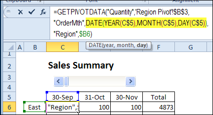
I also used this technique in my Select Date with Excel Scroll Bar example, and you can download a sample file to see how it works.

dateslider14

More on GetPivotData

For more GetPivotData examples, please see my Contextures website: GetPivotData Function

_______________