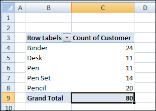
After you create an Excel pivot table, you might want to know how many unique customers placed an order for each product. However, when you add the Customer field to the pivot table’s Value area, it shows the number of orders, not the number of unique customers.
[Note: In Excel 2010 you can use PowerPivot to create a unique count]

Unfortunately, a pivot table doesn’t have a built-in function to calculate a unique count. As a workaround, you could add a column to the source data, then add that field to the pivot table.
Add a Field to the Source Data
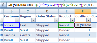
In this example, we want to count the number of unique Customer who ordered each product. We’ll add a column to the pivot table source data, with the heading ‘CustProd’.
In the CustProd column , we’ll enter a formula that refers to the customer (B) and product (E) columns.
=IF(SUMPRODUCT(($B$2:$B2=B2)*($E$2:$E2=E2))>1,0,1)

With this formula, if the row contains the first instance of a customer/product combination, the result is 1. For subsequent instances, the result is 0.
Add the Field to the Pivot Table
After you create the new field in the source data, copy the formula down to the last row of data.
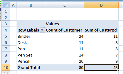
Then add the CustProd field to the pivot table Values area using the Sum function. In the screenshot below, you can see the Sum of CustProd field.

Based on the new CustProd field, we can see that 11 unique customers placed orders for a Binder, and only 7 unique customers ordered a Pen Set.
Video: Show Distinct Count in Excel 2013 With PowerPivot
[Update] To see the steps for setting up the pivot table, and creating the formula, please watch this video.
Video: Count Unique in Excel Pivot Table
[Update]In this short video, I show how to count unique items (distinct count) in a Microsoft Excel pivot table. This method works in Excel 2013 and later versions.
_______________

Hi. many thanks for this tip it helped solve a tricky problem. Now I’m getting greedy! How would I show two dimensions of ‘uniqueness’? If I have 3 products and multiple customers, in multiple sales regions how would I show how many unique customers in london bought pencils and binders. I tried adding another column to the source data that used customer and product as the SumProduct arrays and I suspect the resulting pivot table is ok but the data is presented in a really confusing way that would make no sense to the casual reader; e.g. it shows 65 customers in london (Good), but the total transactions add up to greater than 65 as some customers bought both products. Hope this makes sense and would appreciate any help! Many thanks.
Thank a lot. Very useful hint !
Hi,
I found your count unique values in a pivot table formula…which was exactly what I was looking to do, however there are lines showing up for a given part number the the ‘sum of the customer count’ shows a value of 0…when I blow this out into it’s own worksheet it does in fact show only 1 line of data against that part number. Why will it not show a qty of 1 which is really what it should be based on how the data is displayed. Can you help?
@Emma, if you see items with 0 sum, you might have applied a filter, so the first item (the one with the 1 result) isn’t visible.
This formula is just a workaround, so it doesn’t adapt to changes, the way the other summarized amounts do.
Hello,
The formual works great, but i tend to want to understand what i use. I do get what the formula does but do not understand how the syntax works.
-what does the following statement cause insside the funtion$Q$2:$Q2=Q2
-why do i need to use th * rather than the , between ($Q$2:$Q2=Q2)*($S$2:$S2=S2)
Thanks
Oliver
@Oliver, the formula looks in the cells starting in row 2, down to the active row. It checks for values that match the value in the current row.
This SUMPRODUCT formula uses only two columns, so the * operator multiplies the TRUE/FALSE results in those columns.
If you’re using SUMPRODUCT with more than 2 columns, you can separate with commas, as shown in the example here:
http://www.contextures.com/xlFunctions01.html#SumProduct
Also, Bob Phillips has good information and examples for SUMPRODUCT:
http://www.xldynamic.com/source/xld.SUMPRODUCT.html
If I wanted the unique count of all the customers instead of 43 in the “Grand Total” column is there a way to achieve this? Thanks
Thanks!! It worked for me..
What if you just want to look for unique values in ONE column?
What if I want to find unique values within a time range?
Lets say that I have in column A multiple dates and in column B multiple records that could be repeated among the dates but I want to find how many unique values were during each day, how would do that ?
Thanks in advance
Debra Dalgleish …thanks for replying to Oliver. It really helped me as well.
Marilyn
Thank you! it is an easy way to work around the problem of counting unique values :O)
thanks. best solution i’ve read.
Yess! Exactly the solution I was looking for! I tried so many other places, but this is the one! Good job and a Big Thanks!
In response to my own question (if anyone cares), just download Powerpivot….it will make your life easier (distinct count and DAX language)
best
Hmmmmm Not sure about this but have tried this and the formula gives me a false rather than a value….
I can’t believe it’s so hard to count unique entries. This workaround does not allow for filtering. I have 10,000 records spanning a year’s worth of data. If I want to see how many unique clients I had in January, this formula doesn’t work. It will only show unique clients for the entire data set. If all of my clients have been with me since the beginning of the data set, then I will show zero unique clients for January of this year, which is incorrect. If I modify the formula to start the count over each month then I am inflating my overall unique count for the year by an unknown factor.
It just amazes me that something so easy for me to do (though tedious) is near impossible to do in Excel. It also amazes me that over the 20 year history of Microsoft Excel, Microsoft has not deemed the “unique entries” problem to be worth addressing… It further amazes me that if I add my clients’ names to the rows, IT SHOWS ME THE UNIQUE ENTRIES!!! So it’s already doing the hard part (finding the unique entries), the problem is that it just won’t count them!!! This totally baffles me!!!
@Ryan, I agree, it should be easy to create a unique count in an Excel pivot table. For now, if you’re using Excel 2010, you can use the PowerPivot add-in, as @D3 mentioned.
You can find instructions in my article Unique Count in Excel Pivot Table With PowerPivot
Ryan,
Just download Powerpivot! that’s all you need to get better pivot tables and actually use the distinct counts and much more, don’t forget that Powerpivot its a Microsoft product developed by the SQL Server Team.
Hope this helps,
It’s quite absurd that Excel pivot tables don’t have a “Count Distinct” function. This is a pretty ubiquitous need in analysis. And this “workaround” is pretty lame, because if you want a distinct occurrance with in a certain time frame, this doesn’t address. Microsoft Excel 2010 = LAME!
Hello,
Waiting also for a built in solution from microsoft, I did implement a distinct count function in pivot with some pivot.
Not the most elegant solution, especially on huge spreadsheets, but does the job by providing a reliable unique count within the pivot ( working with multiple dimensions)
Regards
Thanks a lot…exactly what I was looking for! Wish Excel had this built into the option for COUNT DISTINCT or something like that! Perhaps with Excel 2013 they now have it…
Will PowerPivot work with a home user – no server?
Brenda,
All you need to use powerpivot is Excel 2010 or later. No server needed.
Let me know if you have any other questions!
Miguel
Oddly, I’ve copied this example exactly, but the formula won’t work. It’s giving me all 1s, right down.
Nevermind, the person asking me to fix their formulas had calculate set to manual. Which gave me a few hours of additional work…
Thanks Debra. Your post really helps.
This is very useful ! Thanks a ton !!
This worked for me as well. I used it to get a count of unique vendors that had submitted invoices for a specific month. I used the formula combination on Vendor # and Submission Month, and when I made it a General data type format, I got the 0s and 1s described above. Nice Tip!
Thank you It’s worked for me