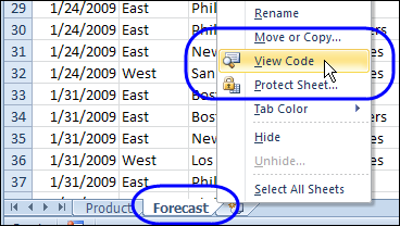
After you add new records to a pivot table’s source data, you’ll have to Refresh the pivot table, to see the new data. See the steps for a pivot table refresh, and how to stop a pivot table refresh. Also, see why other pivot table will refresh at the same time, and how to prevent that from happening.
Continue reading “Stop a Pivot Table Refresh”
Category: Refresh
Manually Clear Old Items in Pivot Drop Down
If you remove an item from your pivot table’s source data, it might still show up in the drop downs, even after you refresh the pivot table.
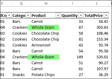
In this example, a product name was originally “Whole Wheat”. In the source data, all the records for that product were changed to the new name, “Whole Grain”.
Continue reading “Manually Clear Old Items in Pivot Drop Down”
Refresh Pivot Table on Protected Sheet
When you protect a worksheet in Excel, you’ll see a list of items that you can allow people to use, while the sheet is protected.
One of those options is ‘Use PivotTable reports’, and if you add a check mark to that option, things might not work exactly as you expected.
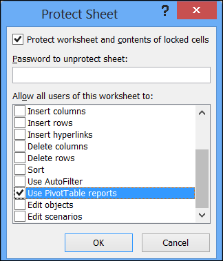
Limited Use of Pivot Tables
When the sheet is protected, even if you have allowed pivot table use, you can’t create a new pivot table. Another restriction is that you won’t be able to refresh a pivot table on the worksheet. If you right-click in a pivot table cell, the Refresh command is disabled.
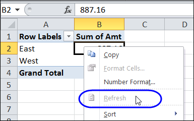
Refresh on Protected Sheet
If you need to refresh a pivot table on a protected sheet, you could
- manually unprotect the worksheet
- refresh the pivot table
- protect the sheet again
Another option, if you would prefer to refresh the pivot table programmatically, is to create a macro that does these steps for you. The following macro will refresh the first pivot table on the active sheet, which has a password – “mypassword”
Sub UnprotectRefresh()
On Error Resume Next

With Activesheet
  .Unprotect Password:="mypassword"
  .PivotTables(1).RefreshTable
  .Protect Password:="mypassword"
End With

End Sub
Connected Pivot Tables
If other pivot tables are connected to the same pivot cache are on protected sheets, you won’t be able to refresh a pivot table, even if it is on an unprotected sheet.
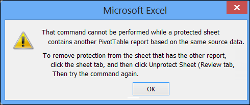
In this situation you will have to unprotect the sheet(s) where those other pivot tables are located, and then do the refresh.
There is sample code to unprotect all the sheets, and do a refresh all, on my Contextures website: Refresh Pivot Table Connected to Protected Sheet
_______________________
Update Pivot Table From Text File
In addition to creating pivot tables from Excel data, you can also use external data sources, such as a text file, like the billing data shown below.
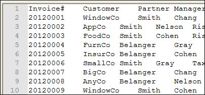
Import the Data
In this example, the billing data was imported to Excel from the text file, onto a worksheet named BillingData. This created an external data range with a connection to the text file.
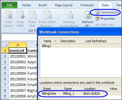
You can create a pivot table based on the imported data, to show a summary of the billing data.
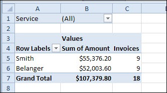
Update the Text File
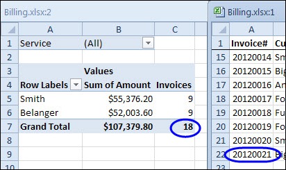
If new billing records are added to the text file, they appear in the external data range when it’s refreshed. However, you might not see the new data in the pivot table that is based on the imported data.
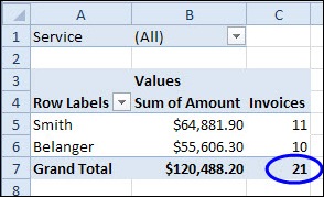
In the screen shot below, there are now 21 invoices in the imported data, but even after refreshing the pivot table, it still shows only 18 invoices. The latest data doesn’t appear in the pivot table.
Use the External Range Name
When you create a pivot table from an external data range, the default data source is a reference to a range of cells, such as BillingData!$A$1:$J$19, where the external data range is located.
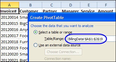
If you use the external data range’s address as the pivot table source, it does not automatically expand, if new data is added to the external data range.
However, when you import external data to an Excel worksheet, a named External Data Range is created, and if you base the pivot table on this named range, it adjusts automatically if records are added or removed.
Change the Pivot Table Source
If a pivot table is based on a specific range of cells, you can change its data source, so it uses the external data range name.
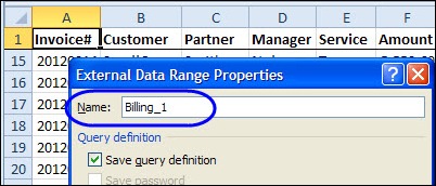
- To see the name of the external data range, right-click a cell in the external data range, and then click Data Range Properties. The range name is shown at the top of the External Data Range Properties dialog box. Click OK to close the dialog box.
- To base the pivot table on this range, select a cell in the pivot table, and then click the Options tab on the Ribbon.
- In the Data group, click Change Data Source.
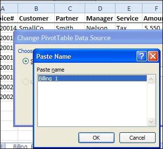
- With the Table/Range highlighted, press the F3 key, and click on the external data range name, e.g. Billing_1
-
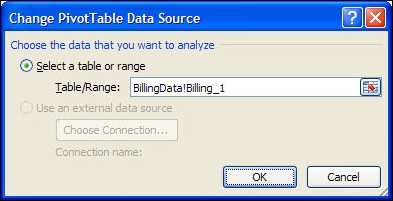
- The Table/Range box will show the sheet name and the external data range name.
- Click OK, to close the Change PivotTable Data Source box.
After the pivot table data source is changed to use the external data source named range, it will update automatically, if data is added or removed.
- Refresh the pivot table to see the new data in the summary.
_______________________
Remove Old Items from Excel 2010 Pivot Table Drop Downs
After you create an Excel 2010 pivot table, the source data may change. New items might be added, and old items are sometimes removed from the data.
In this example, the East and Central regions are merged, and the Central region name is replaced by “East” in all the source data records.
After changing the data, if you refresh the pivot table, the Central region data disappears, but its name is still in the Region drop down.
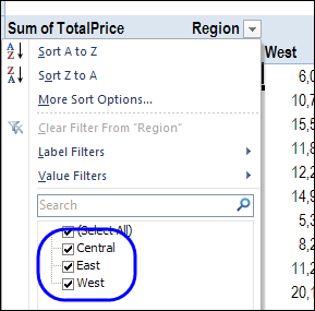
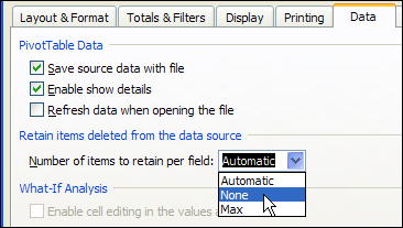
To fix the problem, you can change the Retain Items setting in the pivot table options, to clear old data from the pivot table drop downs.
Watch the Video
To see the steps for preventing old items from appearing in the pivot table, please watch this short video tutorial. These instructions apply to both Excel 2010 and Excel 2007.
__________________________
Excel Pivot Table: Refresh Automatically With Macros
When you update a pivot table’s source data in Excel, the pivot table does not update automatically. You can set the pivot table to update when the Excel file opens, but that doesn’t help if you’re making changes after the file opens. If you can use macros in your Excel file, you can use an event procedure to force the pivot table to refresh automatically if the source data changes.
Continue reading “Excel Pivot Table: Refresh Automatically With Macros”
Improve Performance When Changing Pivot Table Layout
If your pivot table is based on a large data source, it might respond very slowly when you add fields or move fields to a different area of the pivot table.
To improve performance, try the following tips:
- Remove any pivot table styles and any other formatting, such as conditional formatting that you applied to the pivot table.
- Calculated items can negatively impact the speed of updating. If possible, remove any fields that contain calculated items, or delete the calculated items from the fields.
Defer Layout Update
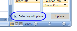
If you plan to add or move more than one field, you can use the Defer Layout Update option. When this feature is enabled, the fields are all added or moved, and then the pivot table is recalculated once. If this box is not checked, the pivot table is recalculated after each field is added or moved.
To defer the layout updates:
- Add a check mark to the Defer Layout Update box in the PivotTable Field List.
- Move or all all the fields that you want to adjust
- Click the Update button, to the right of the Defer Layout Update check box.
- When you’re finished changing the layout, remove the check mark from the Defer Layout Update check box.
Note: Some features, such as filtering and grouping, are not available when Defer Layout Update is activated.
_____________
Refreshing All Pivot Tables in a Workbook
If there are several pivot tables in your workbook, you might want to refresh all of them at the same time instead of refreshing each pivot table individually.
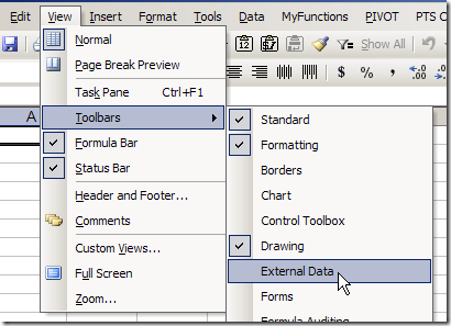
To refresh all the pivot tables in the active workbook at the same time, display the External Data toolbar, and click the Refresh All button.
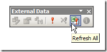
Note: Using the Refresh All command will also refresh all external data ranges in the active workbook, and affects both visible and hidden worksheets.
Display the External Data Toolbar
- Click the View menu
- Click Toolbars, then click External Data
Add the Refresh All Button to the PivotTable Toolbar
Instead of displaying the External Data toolbar, you can add the Refresh All button to the PivotTable toolbar:
- Select a cell in a pivot table, then click the Toolbar Options arrow at the end of the PivotTable toolbar.
- Click Add or Remove Buttons

- Click Pivot Table.

- Click Refresh All to select it (a checkmark will appear beside each selected button).
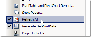
- Click outside the list to close it.
- ___________________________
For more information on pivot tables, see the Pivot Table Topics on my Contextures web site.
___________________________
Automatically Include New Data in a Pivot Table
If your pivot table is based on Excel data, you probably add new records to that data, on a regular basis. You want the pivot table to automatically include those new records, without you having to manually change the pivot table range every time you add new data.
A range that expands automatically is called a dynamic range, and here are a couple of ways to create one in Excel.
Create a Named Table
In Excel 2010 and 2007, you can format a list as a Named Table, and use that as a dynamic source for your Pivot Table. There are instructions here: Excel Tables — Creating an Excel Table. This is a quick and easy way to create a dynamic range.
Create a Dynamic Range With a Formula
In Excel 2007, and earlier versions, you can use a formula to create a dynamic range, which will automatically expand to include any new rows and columns. Follow these steps to create a dynamic range:
- Select the top-left cell in the source table. This step isn’t necessary, but helps you by inserting the cell reference in the name definition.
- Choose Insert | Name | Define.
- In the Names in workbook box, type a name for the dynamic range, for example, PivotData.
- In the Refers to box, type an OFFSET formula that refers to the selected cell. For example, with cell A1 selected on a worksheet named Pivot, you’d type (all on one line)
=OFFSET(Pivot!$A$1,0,0,
COUNTA(Pivot!$A:$A),
COUNTA(Pivot!$1:$1)) - Click the OK button.
Change the Pivot Table Source
Then, change the pivot table’s source to the dynamic range that you created:
- Right-click a cell in the pivot table.
- On the shortcut menu, click PivotTable Wizard.
- Click the Back button.
- In the Range box, type the name of the dynamic range, and click Finish.
Note
This technique will not work if there are other items in row 1 or column A of the Pivot worksheet. Those items would be included in the count, and would falsely increase the size of the source range.
______________
Locate Source Data For a Pivot Table
You might have to make changes to a workbook that contains a pivot table. If someone else created that workbook, you may not be sure where to find the Excel table that was used as the pivot table’s source data. In some workbooks there can be several Excel tables, and it’s not immediately obvious which table was used. These tips will help you locate the source data for a pivot table.

