Category: Refresh

After you create an Excel pivot table, the source data usually changes. New records are added, and old records might be changed or deleted.

Later, when you refresh the pivot table, you should see a summary of your updated data, but sometimes there’s a problem – old data sticks in the drop down lists.

Example: Region Names Changed

To show this pivot table problem, I made short video, which you can see in the next section.

My sample file has data from a fictional sales company, and the source data was changed:

• Central region was merged into the East region.
• Sales records were changed from Central to East

After making those changes, I refreshed the pivot table. As expected, the Central region’s name disappeared from the Region headings.

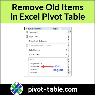
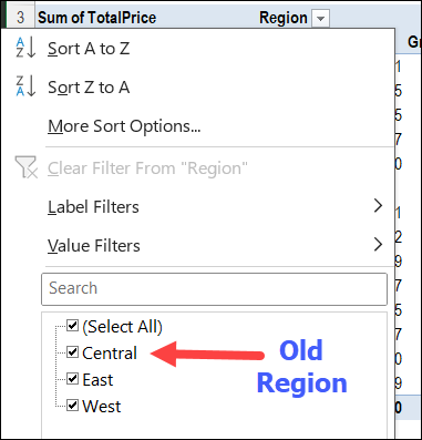
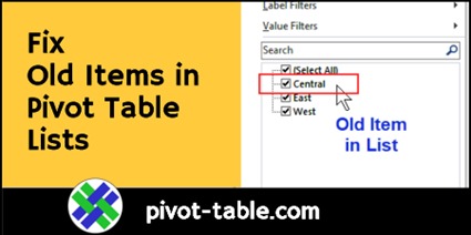
However, Central still shows up in the Region drop down.

Video: Clear Old Pivot Table Items

In this short video, I show how you can clear the old Region name from the pivot table drop down list.

Doing this will also prevent old items from appearing in this pivot table, in the future.

Video: Clear Old Items – Default Settings

In Excel 365, and Excel 2019, it’s even easier to avoid old items in pivot table drop downs.

Instead of changing this setting for every pivot table that you create, you can change it once, in your Excel default settings for Pivot Tables.

In the video below, I show the steps for changing an individual pivot table, like I did in the previous video.

Then, at the 2:57 mark, I show how to change the default setting, in Excel 365. You can skip to that section, if you’d like!

Prevent Old Items in Pivot Table

To stop old items from showing in an existing pivot table, follow the steps below.

NOTE: This setting will affect all the pivot tables that use the same pivot cache.

• First, right-click a cell in the pivot table
• Next, in the right-click pop-up menu, click on PivotTable options
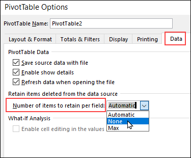
• In the PivotTable Options dialog box, click on the Data tab
• In the Retain Items section, there is a drop down for “Number of items to retain per field”
  • By default, that is set to Automatic.
• Click the drop down arrow, and select None from the drop down list.
• Click OK, then refresh the pivot table.

Get the Excel Workbook

To get the sample file, go to the Clear Old Items page on my Contextures site.

That page also has Excel macros that you can use, to

• change the Retain Item settings for all pivot tables in the workbook
• change Excel’s default settings for pivot tables (Office 365 or Excel 2019 and later)

More Pivot Table Tutorials

Show and Hide Pivot Items

Refresh Pivot Table

Grouping Data

Pivot Filters, Multiple

Pivot Filter Macros

_______________________

Remove Old Items – Excel Pivot Table Drop Down

_______________________

In a perfect world, if you need to make a pivot table, the data is nicely organized in a table, and you can connect to that, quickly and easily.

Unfortunately, as you know, things aren’t  always perfect, especially when it comes to data! And sometimes the data is in two or more separate tables, so you need to combine it somehow, before you can build a pivot table..

4 Ways to Combine Data for Pivot Table

There are different ways you can combine data from multiple tables in Excel. For example:

1. Power Query
2. VSTACK Formula
3. Excel Macros
4. Pivot Table Wizard

Combine Data Videos

In the sections below, there are a couple of short “Combine Data” videos that I’ve made recently.

• The first video shows how to use the VSTACK function, which is available in Excel 365. It returns multiple ranges in a vertical stack, so it’s easy to combine tables that have identical structures.
• The second video shows how to combine data using the old Pivot Table Wizard. It creates a pivot table with several limitations, but it might do what you need – if you don’t need anything fancy!

For all 4 methods, you can find detailed steps, and sample files, on my Contextures site, on the Pivot Table from Multiple Sheets page .

Video: Create Pivot Table from 2 Tables

Here’s the VSTACK function video, in which I combine the data from tables on 2 separate worksheets. It only takes one cell with a formula, to return all the data from the two tables.

I included the headings for the first table too, because pivot table data needs headings!

Video Timeline

• 00:00 Pivot Table from Multiple Sheets
• 00:20 VSTACK Function
• 00:52 VSTACK Formula
• 01:21 Combined Data
• 01:39 Named Range
• 02:11 Add Pivot Table

Pivot Table Wizard

What if you don’t have Power Query, or the Excel VSTACK function. And you don’t want to use Excel macros?

In that case, you can use the old Pivot Table Wizard to do the job. It’s well hidden in newer versions of Excel, but in the video, I’ll show you how to open it, with an Excel keyboard shortcut.

Video Timeline

• 0:00 Data on 2 Sheets
• 0:24 Open PivotTable Wizard
• 0:50 Select Sheet Ranges
• 1:08 Page Field Settings
• 1:29 Adjust the Pivot Table
• 2:04 Show Sum
• 2:15 Page Field

Get the Sample File

For all 4 methods to combine data, you can find detailed steps, and sample files, on my Contextures site.

Follow this link, to go to the Pivot Table from Multiple Sheets page .

____________________________

4 Ways to Build Pivot Table from Multiple Sheets

____________________________

With a large pivot table, running a macro that refreshes that pivot table might be painfully slow. The usual macro steps, like turning off screen updating, and disabling events, don’t solve this problem. Try adding an extra bit of code to your macro, to see if that makes the refresh go faster.

Continue reading “Faster Pivot Table Refresh in Excel Macros”

A simple data change can cause a strange pivot table refresh error, if you added the data to the Data Model. The long error message starts with, “We couldn’t get data from the Data Model. Here’s the error message we got”. It also mentions “function PCMinorObjectCollection”, which I’d never heard of before. See what causes this problem, and how to fix it.

Continue reading “Excel Data Model Pivot Table Refresh Error”

When you create a pivot table in Excel, it includes all the source data, even if some rows were hidden by filtering. However, if you’re using a version of Excel that has the new Spill (dynamic) functions, you can try this technique, to create a pivot table from filtered list visible rows only

Continue reading “Pivot Table from Visible Rows in List”

After you create a pivot table, you might add or change records in the source data. When you refresh the pivot table later, sometimes the new data doesn’t show up. Here’s how to find and fix the pivot table source data, so the correct data appears.

Continue reading “Find and Fix Pivot Table Source Data”

If you remove items from a pivot table’s source data, those items might still appear in the pivot table drop down lists, even after you refresh the pivot table. Here’s how you can stop those old items from appearing – watch the short video, or read the written steps below.

Continue reading “Fix Old Items in Excel Pivot Table Lists”

When you protect a worksheet, you can add a check mark in the options list, to allow the use of pivot tables and pivot charts. However, even with that option turned on, you can’t refresh an Excel pivot table on a protected sheet. Use this macro to turn off the protection and update the pivot table.

Continue reading “Refresh an Excel Pivot Table on a Protected Sheet”

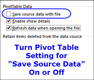
When you create a pivot table in your workbook, the source data records are saved in a special memory area – a pivot cache.  Then, when you close the file, Excel can save the source data in this pivot cache, or clear that memory.

Keep reading, to see how you can change this setting, and learn the advantages and disadvantages of either choice.

Note: If you want to re-create the source data, see: Re-create the Source Data

Continue reading “Saving Source Data with Pivot Table File”

It would be nice to automatically refresh an Excel pivot table, whenever its source data changes. Unfortunately, there isn’t a built-in way to make that happen. However, here are 3 ways you can refresh a pivot table, after you make changes to the source data.

Continue reading “Automatically Refresh an Excel Pivot Table”