Category: Excel Pivot Table

The Excel PivotPower add-in on the Contextures website has been updated.

The PivotPower add-in makes it easier to change the summary functions in a pivot table, or add protection, and has several other helpful commands.

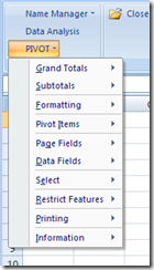
After you install the add-in, it shows up as a drop down list on the Excel Ribbon’s Add-Ins tab. In older versions of Excel, the add-in creates a PIVOT menu on the Excel menu bar.

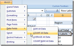
You can select a cell in a pivot table, and run a command, so the changes only affect the selected pivot table.

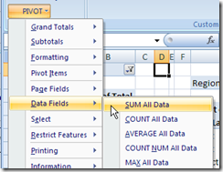
Or, select a cell that isn’t in a pivot table, and the command will change all the pivot tables on the active sheet.

To download the file, you can go to the PivotPower Add-In page on the Contextures website. You’ll find installation instructions and details on the PivotPower commands.

___________

For a pivot table that’s based on a Microsoft Access query, you might need to find out which database and query were used as the source data.

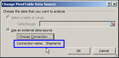
In Excel, if you click the Change Data Source command, on the Ribbon’s Options tab, you can see the connection name in the Change PivotTable Data Source dialog box. However, that bit of information isn’t too useful — it doesn’t show you the name and path of the Access file, and you can’t see which query was used to create the pivot table.

 

View the Connection Properties

To find the details on the source data’s Access file and query, you can follow these steps:

• In the Excel file, select a cell in the pivot table
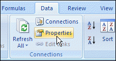
• On the Ribbon’s Data tab, in the Connections group, click Properties.

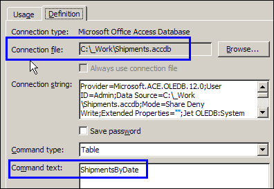
• In the Connection Properties dialog box, click the Definition tab.
  • In the Connection File box, you can see the name and path of the database.
  • In the Command Text box is the name of the Access query.
• Click Cancel to close the Connection Properties dialog box.

______________

In Excel 2010, you can use the free PowerPivot add-in to create a report from multiple Excel workbooks or worksheets. With PowerPivot, it’s easy to connect the tables using the Primary and the Foreign key, such as ‘ProductID’ in a Sales table and a Pricing table.

In some cases though, you might want to combine the data in two Excel files, or worksheets, that have an identical structure. For example, you could have sales data for the different regions, or expense data for multiple years.

Because the tables have identical structures, you can’t use a key to connect them; instead, you would need to create one combined table from all the data. The technique shown in the following video allows you to import more than a million records from Excel, despite the fact that one worksheet can only contain up to 1,048,576 rows.

Thanks to Excel MVP, Kirill Lapin, for sharing this very helpful tip. You can see more of Kirill’s work in the Contextures Blog post on Combining Data from Two Excel Files in a Pivot Table.

Detailed Instruction and Sample Files

To see detailed instructions for this technique, with more screen shots, visit the PowerPivot from Identical Structure Excel Files page on the Contextures website. That page also has a link for downloading the East and West sales data that I used in this example.

Watch the PowerPivot Video

To see the steps for combining data from multiple tables in PowerPivot, please watch this video.

Download the PowerPivot Add-In

You can download the free PowerPivot add-in from the Microsoft website: PowerPivot Download

__________

The Pivot Table Wizard isn’t available on the Ribbon in Excel 2007. To open the Pivot Table Wizard, you can use the keyboard shortcut — Alt + D, P — as described in the article on creating a pivot table from multiple sheets.

Another option is to add the Pivot Table Wizard button to your Quick Access Toolbar (QAT), by following the steps below.

Customize the QAT

To add the Pivot Table Wizard to your QAT, follow these steps:

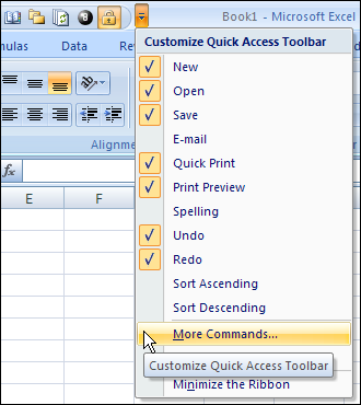
• Click on the Customize Quick Access Toolbar button
• Click More Commands

 

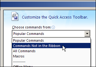
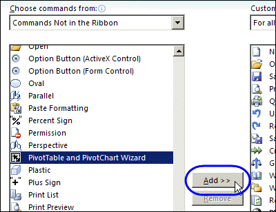
• From the ‘Choose commands from’ drop down list, select ‘Commands Not in the Ribbon’

 

• In the list of commands, click PivotTable and PivotChart Wizard
• Click the Add button, then click OK

Open the Pivot Table Wizard

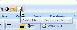
Now that the Pivot Table Wizard button has been added to the QAT, you can click it to open the Pivot Table Wizard.

 

___________

Sometimes it’s quicker to use a keyboard shortcut, instead of the mouse, to accomplish a task in Excel. Here are some of the keyboard shortcuts for working with pivot tables in Excel 2007 and Excel 2003.

Excel 2007 Pivot Table Keyboard Shortcuts

Shortcut	Action
Ctrl + Shift + *	Select entire pivot table (not including Report Filters)
Ctrl +  A	Select entire pivot table (not including Report Filters)
Spacebar	Add or remove checkmark for selected field in PivotTable Field List
Alt + Shift + Right Arrow	Group selected pivot table items
Alt + Shift + Left Arrow	Ungroup selected pivot table items
Down Arrow	Select next item in PivotTable Field List or Items List
Up Arrow	Select previous item in PivotTable Field List or Items List
End	Select last item in PivotTable Field List or Items List
Home	Select first item in PivotTable Field List or Items List
Alt + Down Arrow	Open field list for active cell
Ctrl + –	Hide selected item or field
Shift + Ctrl + =	When data field selected, opens Calculated Field dialog box
Shift + Ctrl + =	When field heading cell selected, opens Calculated Item dialog box
Alt + D, P	Open the old PivotTable Wizard

 

Excel 2003 Pivot Table Keyboard Shortcuts

In Pivot Table

Shortcut	Action
Alt + L	Show Pivot Table dialog box
Alt + R	move selected field into Row area
Alt + D	move selected field into Data area
Shift + Right Arrow	Group selected pivot table items
Alt + Shift + Left Arrow	Ungroup selected pivot table items
Down Arrow	Select next item in Items List
Up Arrow	Select previous item in Items List
End	Select last visible item in List
Home	Select first visible item in List
Alt + Down Arrow	Open field list for active cell
Ctrl + –	Hide selected item or field
Shift + Ctrl + =	When data field selected, opens Calculated Field dialog box
Shift + Ctrl + =	When field heading cell selected, opens Calculated Item dialog box

In Pivot Table Wizard

Shortcut	Action
Alt + C	move selected field into Column area
Alt + R	move selected field into Row area
Alt + D	move selected field into Data area
Alt + P	move selected field into Page area

_____________

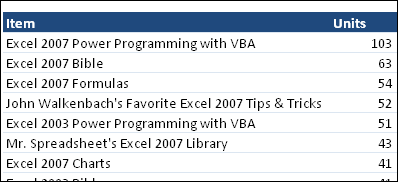
This week, John Walkenbach, aka Mr. Spreadsheet, used a pivot table report to analyze his website’s Amazon sales for 2009. Here’s a screenshot of the results, showing the top sellers, and number of units sold.

John knows a thing or two about Excel, having written over 40 Excel books, so take a look at the full list, and see if there’s something there that will help you.

Excel 2007 Power Programming with VBA

I bought a copy of John’s Excel 2007 Power Programming with VBA a couple of years ago, and highly recommend it. The book is a great reference when you’re learning VBA, or upgrading from an earlier version of Excel.

In its 1104 pages, the book covers pretty much everything you need to know about Excel VBA, and comes with a CD that contains:

• Sample files for the book’s VBA tutorials
• A searchable PDF version of the book

And best of all, there’s a chapter on Pivot Table Programming, that will help you get started with the new pivot table features in Excel 2007. In that chapter, you’ll discover what’s new in Excel 2007 pivot tables, and learn how to:

• create pivot tables with VBA
• create a complex pivot table
• create multiple pivot tables
• use VBA to change a summary table to a worksheet table

_____________

Chandoo, at the Pointy Haired Dilbert blog, has posted 5 Excel Pivot Table tricks today. His blog posts are always informative and entertaining, so go and take a look.

The 5 Pivot Table tricks are:

1. Drill Down Pivot Tables
2. Change Summary from Total
3. Slice and Dice Pivots
4. Difference from Last Month
5. Calculated Fields in Pivots

Did you know all those pivot table tricks? Learn anything new?

______________

For more information on Pivot Tables, please see the Pivot Table Tutorials on the Contextures Website.

______________

NOTE: This contest ended in 2010, and link is no longer owned by the PowerPivot team.

The team at PowerPivot for Microsoft Excel 2010 created the Excelerators Quiz, where you can test your Excel skills. To make the challenge more exciting, they’re sponsoring a giveaway on the Contextures blog (for USA residents only).

The blog giveaway prize has a total value of over $250, and will include a Dell ST2310 23 inch flat panel monitor, keyboard, and mouse.

How to Enter

To enter the giveaway, after you take the Excelerators Quiz, go to the Contextures blog, read the rules, and add a comment. In your comment:

• Create your own unique question for the Excelerators Quiz.
• Make your question multiple choice, with the correct answer as one of the four options.

The Alpha Geek Challenge

The PowerPivot team has also launched an Alpha Geek Challenge for more advanced excel geeks. Donald Farmer will host a PowerPivot competition in which the Grand Prize winner will receive an all-expenses paid trip to the 2010 Microsoft BI Conference in New Orleans, LA in June.

After you finish the Excelerators Quiz, and enter the Contextures blog giveaway contest, see how you do in the Alpha Geek Challenge!

_____________