Pivot Table Calculated Field: Tasks Per Hour

Instead of creating formulas in the source data for your pivot tables, you can create formulas in the pivot table, by using calculated fields and calculated items.

In this example, we’ll create a calculated field, to show the number of tasks per hour that are completed by each worker.

Continue reading “Pivot Table Calculated Field: Tasks Per Hour”

Use Pivot Table Calculated Item

If you need to sum specific items in a pivot table field, you can create a calculated item. For example, if your pivot table contains an Order Status field, with four types of status:

  • Shipped
  • Pending
  • Backorder
  • Canceled

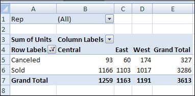
You could create a calculated item, named Sold, that sums the units sold, for orders with a status of Shipped, Pending, or Backorder.

Create a Calculated Item

Follow these steps to create a calculated item:

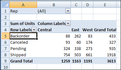
  1. In the pivot table, select a cell that contains an Order Status item. For example, select cell A5, that contains the Backorder item.calculateditem01
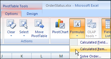
  2. On the Ribbon’s Options tab, in the Tools group, click Formulas, and then click Calculated Item.calculateditem02
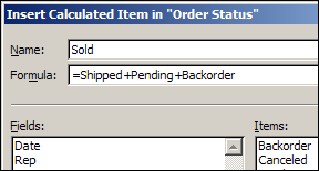
  3. Type a name for the Calculated Item, for example, Sold, and then press the Tab key to move to the Formula box.
  4. In the Fields list, select Order Status, and in the Items list, double-click Shipped, and then type a plus sign (+).
  5. Double-click Pending, type a plus sign, and then double-click Backorder. The complete formula is =Shipped+Pending+Backorder.calculateditem03
  6. Click OK, to save the calculated item, and to close the dialog box.

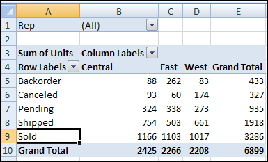
The new calculated item, Sold, is added to the Row area in the pivot table. However, the Grand Totals have increased, because the Sold item includes the values from other items.

calculateditem04

Hide the Unnecessary Pivot Items

In the pivot table, you can hide the Shipped, Pending, and Backorder items, because they are included in the Sold calculated item.

calculateditem05

With those pivot items hidden, the pivot table will show the correct Grand Totals.

calculateditem06

Download the Sample File

To see the pivot table data and the calculated item, you can download the sample file from the calculated item page on my Contextures website.

In the Download section, click on the first item — Create a Calculated Item sample file.

The file is in xlsx format, and is zipped.

_______________

Pivot Table Summary Functions: StdDev and StdDevp

Previously, we’ve looked at the pivot table summary functions:  Count, Average, Min and Max and Product. In this article we’ll look at the StdDev and StdDevp summary functions.

StdDev Function and StdDevp Function

Like the STDEV.P and STDEV.S worksheet functions, the StdDev and StdDevp summary functions calculate the standard deviation for the underlying data in the Values area, and is the square root of the variance. Like the variance, standard deviation is a measure of how widely the values vary from the average of the values.

The StdDevp summary function is used when the entire population is used in the calculation. If a sample of the data is used, instead of the entire population, then use the StdDev summary function.

STDEV.P Worksheet Function

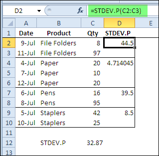
Shown below is the pivot table source data, and the STDEV.P worksheet function is calculating the standard deviation for each product type. There is a large difference between the quantities of file folders sold, and the standard deviation is 44.5. For the paper sales, the difference in quantity is much smaller, and the standard deviation is only 4.71.

pivotstdev00 

Pivot Table StdDevp Summary Function

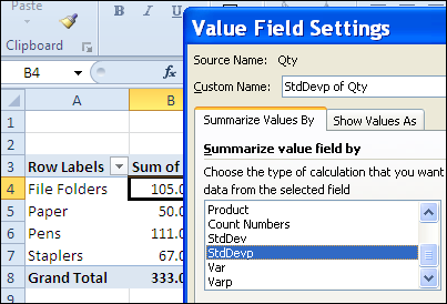
To use the StdDevp summary function, when the Qty field is added to the pivot table, change the summary calculation to StdDevp.

pivotstdev01b 

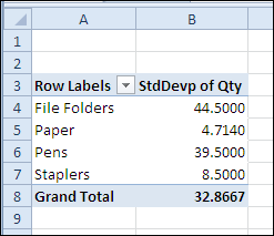
The standard deviations shown in the pivot table are the same as those that were calculated on the worksheet.

 pivotstdev02  

Note: If the count of items is one, a #DIV/0! error is displayed when using the StdDev summary function, because one is subtracted from the count when calculating the standard deviation.

How the Standard Deviation is calculated

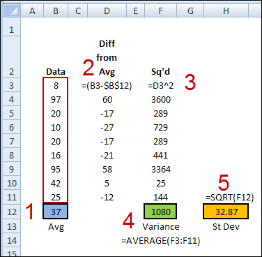
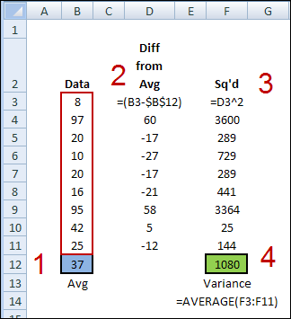
In the standard deviation, each number is compared to the mean of the numbers. If you were to calculate the standard deviation on the worksheet, without the STDEV.P function, here’s how you would do it.

  1. Find the average of the numbers in the pivot table data.
  2. From each number, subtract the average.
  3. Square the calculated difference for each number
  4. Find the average of the squared difference.
  5. Find the square root of the average.

pivotstdev03 

_______________

Pivot Table Summary Functions: Var and Varp

Previously, we’ve looked at the pivot table summary functions:  Count, Average, Min and Max and Product. In this article we’ll look at the Var and Varp summary functions.

Var Function and Varp Function

Like the VAR.P and VAR.S worksheet functions, the Var and Varp summary functions calculate the variance for the underlying data in the Values area, and is the square of the standard deviation. Like the standard deviation, variance is a measure of how widely the values vary from the average of the values.

The VarP summary function is used when the entire population is used in the calculation. If a sample of the data is used, instead of the entire population, then use the Var summary function.

VAR.P Worksheet Function

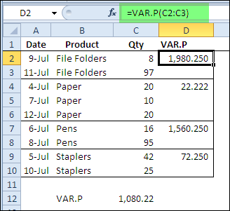
Shown below is the pivot table source data, and the VAR.P worksheet function is calculating the variance for each product type. There is a large difference between the quantities of file folders sold, and the variance is 1980.25. For the paper sales, the difference in quantity is much smaller, and the variance is only 22.22.

pivotvarp00

Pivot Table Varp Summary Function

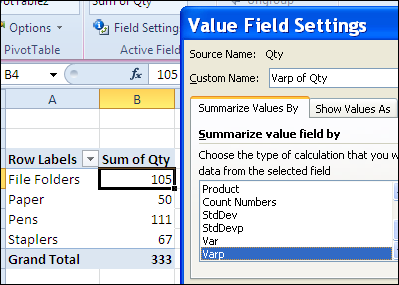
To use the Varp summary function, when the Qty field is added to the pivot table, change the summary calculation to Varp.

pivotvarp01b

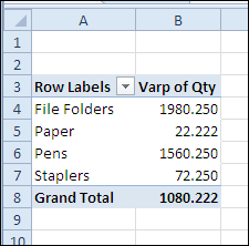
The variances shown in the pivot table are the same as those that were calculated on the worksheet.

pivotvarp02  

Note: If the count of items is one, a #DIV/0! error is displayed when using the Var summary function, because one is subtracted from the count when calculating the variance.

How the Variance is calculated

In the variance, each number is compared to the mean of the numbers. If you were to calculate the variance on the worksheet, without the VAR.P function, here’s how you would do it.

  1. Find the average of the numbers in the pivot table data.
  2. From each number, subtract the average.
  3. Square the calculated difference for each number
  4. Find the average of the squared difference.

pivotvar03

_______________

Pivot Table Summary Functions: Product

In recent blog posts, we’ve looked at the pivot table Count function, the Average function, and the Min and Max functions. In this article we’ll look at the Product function.

Product Summary Function

The Product summary function shows the result of multiplying all the underlying values in the Values area. The result is the same as using the PRODUCT function on the worksheet to calculate the multiplied values.

In all the years that I’ve worked with pivot tables, I’ve never had to use the Product summary function, and can’t imagine a situation where it would be useful. However, you can see how it works, and decide if it would be useful in any of your applications.

PRODUCT Worksheet Function

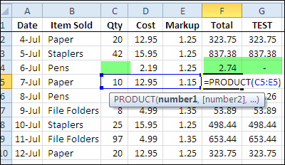
The PRODUCT worksheet function can be useful as a quick way to multiply several values in a worksheet row. For example, in this list of orders, the PRODUCT function multiplies the item quantity, times the cost, times the markup rate, to get the total price for each order.

In column G, you can see the total calculated by using the multiplier operator instead. The only case in which the results are different is where there is a blank cell, such as in row 4. The PRODUCT function treats the blank as a 1, and the multiplier operator treats the blank as a zero.
pivotproduct02 

In this scenario, the PRODUCT worksheet function shows a meaningful result.

PRODUCT Worksheet Function for Columns

However, when you’re using data  as the source for a pivot table, you aren’t multiplying rows, as you would with the PRODUCT worksheet example above. The pivot table will summarize the data from several, or even thousands of rows, so the PRODUCT function isn’t useful, in my experience.

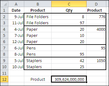
In the screen shot below, you can see the pivot table source data, with the product calculated for each type of item that’s sold, using the PRODUCT worksheet function. Instead of multiplying the values in rows, values in the same column (Qty) are being multiplied.

At the bottom of the source data is the overall PRODUCT calculation.
pivotproduct01

Unlike the previous example, these products are meaningless.

Pivot Table Product Summary Function

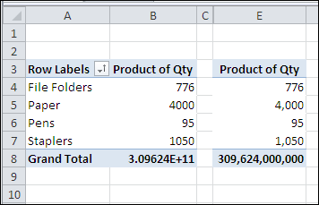
When you use the Product summary function in a pivot table that’s based on the data source shown above, the results are the same meaningless numbers.

The results of the Product function may be very large numbers and default to a Scientific number format. You can format the numbers as Number format, instead of Scientific format.

Note: Excel only stores and calculates with 15 significant digits of precision, so after the 15th character you’ll only see zeros.
 pivotproduct03

_________
Pivot Table Summary Functions: Max and Min

In recent blog posts, we’ve looked at the pivot table Count function and the Average function. Now we’ll look at two more functions, that are closely related — Min and Max.

Max Summary Function

The Max summary function shows the maximum value from the underlying values in the Values area. The result is the same as using the MAX function on the worksheet to calculate the maximum of the values.

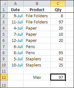
In the screen shot below, you can see the source data for a small pivot table, and the maximum quantity, using the worksheet’s MAX function, is 97.

pivotmax01

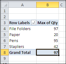
With a pivot table, you can quickly see the maximum for each product that was sold, and the grand total — 97 — which matches the worksheet maximum.

pivotmax02

Min Summary Function

The Min summary function shows the minimum value from the underlying values in the Values area. The result is the same as using the MIN function on the worksheet to calculate the minimum of the values.

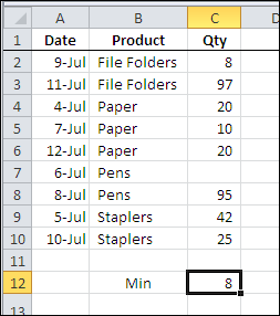
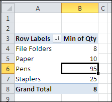
In the screen shot below, you can see the source data for a small pivot table, and the minimum quantity, using the worksheet’s MIN function, is 8.

pivotmin01

With a pivot table, you can quickly see the minimum for each product that was sold, and the grand total — 8 — which matches the worksheet minimum.

pivotmin02

In both the worksheet and the pivot table, the blank cell is ignored when calculating the minimum amount.

___________


___________
Pivot Table Summary Functions: Average

When you add a numeric data field to the Values area in a pivot table, the summary function defaults to either Sum or Count. You can change that field to use one of the other summary functions, such as Average.

The Average Function

The Average function in a pivot table works like the AVERAGE function on the worksheet to calculate the average (mean) of the values. It totals all the underlying values in the Values area, and divides by the number of values. 

pivottableaverage05 

You can use the Average function to compare amounts, such as order sizes, student grades, and project times, across a large number of instances.

Blanks and Zeros

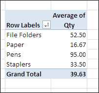
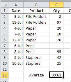
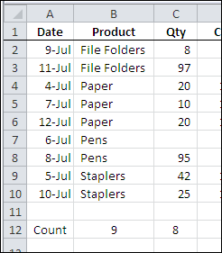
Just as they are on the worksheet, blank cells are ignored when calculating the pivot table averages, but zero cells are included.

In the data source shown below, cell C7 is blank. That blank cell is not included in either the worksheet average (C12),

pivottableaverage01

or in the pivot table average, shown below.

pivottableaverage05 

Hidden Zeros

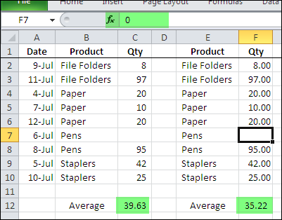
If you have formatted the worksheet to hide zero values, remember that those zero values will be included in the averages, even if the cells appear blank.

In the two data sources shown below, the overall average is different. Zeros are hidden on the worksheet, and cell F7 contains a zero. Cell C7 is blank.

pivottableaverage04

If you create pivot tables from these two data sources, the pivot table Average function would include the hidden zeros, just as the worksheet Average does.

Format the Results

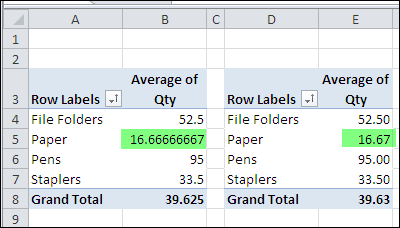
When you use the Average summary function, the results will probably show a strange mixture of decimal places, as shown in the pivot table at the left, in the screen shot below.

pivottableaverage03

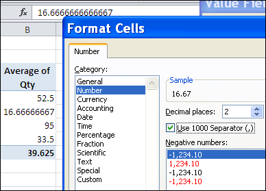
Format the field to have a consistent number of decimal places (as in the pivot table at the right, above), so the numbers are easy to compare.

pivottableaverage02

____________

Pivot Table Summary Functions: Count

When you add a field to a pivot table’s Values area, Count is the default summary function, if the field contains nonnumeric or blank cells. (If the field’s data are all numbers, Sum is the default function.)

The Count function’s name is slightly confusing, because it’s like the COUNTA worksheet function, not the COUNT worksheet function.

The pivot table Count function counts:

  • text
  • numbers
  • errors

Blank cells are not counted.

Watch What You Count

If you’re using the Count function in a pivot table, be careful which field you use for the count. For example, in the pivot table source  data shown below, cell C7, in the Qty column, is blank.

pivottablecount01

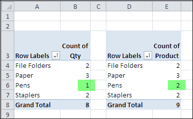
if you want to count the order for Pens, and use the Qty field, the blank cell (C7) would not be counted. The number of orders for Pens would show as 1. Instead, you could add the Product field to the Values area, and the Pens orders would show a count of 2.

In the pivot tables shown below, the one on the left uses Qty in the Values field, and the pivot table on the right uses Product in the Values field.

pivottablecount02

__________

Create an Excel 2007 Pivot Table and Show Averages

This example is based on the Work Orders workbook, used in my book, Beginning PivotTables in Excel 2007.

If you’re working through the book, this video shows the steps outlined starting on page 46.

In the video, we create a pivot table that’s based on a formatted Excel Table.

Then, the Values field is changed from SUM to AVERAGE, and the numbers are formatted so they’re easy to read and understand.

___________________

Count Unique Items in an Excel Pivot Table

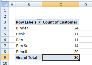
After you create an Excel pivot table, you might want to know how many unique customers placed an order for each product. However, when you add the Customer field to the pivot table’s Value area, it shows the number of orders, not the number of unique customers.

[Note: In Excel 2010 you can use PowerPivot to create a unique count]

CountUnique01

Unfortunately, a pivot table doesn’t have a built-in function to calculate a unique count. As a workaround, you could add a column to the source data, then add that field to the pivot table.

Add a Field to the Source Data

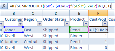
In this example, we want to count the number of unique Customer who ordered each product. We’ll add a column to the pivot table source data, with the heading ‘CustProd’.

In the CustProd column , we’ll enter a formula that refers to the customer (B) and product (E) columns.

=IF(SUMPRODUCT(($B$2:$B2=B2)*($E$2:$E2=E2))>1,0,1)

CountUnique02

With this formula, if the row contains the first instance of a customer/product combination, the result is 1. For subsequent instances, the result is 0.

Add the Field to the Pivot Table

After you create the new field in the source data, copy the formula down to the last row of data.

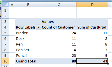
Then add the CustProd field to the pivot table Values area using the Sum function. In the screenshot below, you can see the Sum of CustProd field.

CountUnique03

Based on the new CustProd field, we can see that 11 unique customers placed orders for a Binder, and only 7 unique customers ordered a Pen Set.

Video: Show Distinct Count in Excel 2013 With PowerPivot

[Update] To see the steps for setting up the pivot table, and creating the formula, please watch this video.

Video: Count Unique in Excel Pivot Table

[Update]In this short video, I show how to count unique items (distinct count) in a Microsoft Excel pivot table. This method works in Excel 2013 and later versions.

_______________