Pivot Table Calculated Field Removed with Excel VBA

If you’re working with pivot table calculated fields in Excel VBA programming, or trying to use the Orientation property for data fields, you might encounter some problems. Here’s how I managed to work around an error that occurs for a pivot table calculated field removed with Excel VBA.

Continue reading “Pivot Table Calculated Field Removed with Excel VBA”

Pivot Table From Data in Multiple Workbooks

To create a pivot table from data on different worksheets, you can use a Multiple Consolidation Ranges pivot table, but the result is a pivot table with limited features and functionality.

Previously, Excel MVP Kirill Lapin shared his macro for creating a standard pivot table from data on different worksheets.

Now Kirill has expanded that technique, and written a macro to build a pivot table from data in multiple Excel files.

Pivot Table Macro

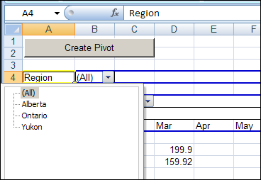
In Kirill’s example, the main file is named Report.xls. It contains the pivot table code, and a button that runs the macro. After you start the macro, it prompts you to select one or more data files, all stored in the same folder.

All of the data files must have the same structure, and the macro pulls the data stored on Sheet1 in each file.

Standard Pivot Table

The macro creates a standard pivot table based on a Union query, and not built from Multiple Consolidation Ranges, it’s a fully functioning pivot table, and you can pivot, group and filter the data, as usual. You can also refresh the pivot table, to show the latest data in the source files, as long as those files stay in their original location.

pivotwkbk04

The Union Query

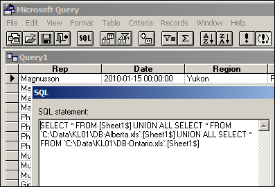
Kirill’s macro creates a Union query to combine the data from all the selected files. If you open Microsoft Query, you can see the SQL string for the Union query, and all the data from the selected workbooks.

pivotwkbk05

Download the Sample File

You can download the Pivot Workbooks example to see the sample code and create the pivot table. The zipped folder that contains the Report.xls file, and the five sample data files. Unzip the folder, and keep all the files in the same folder. When you open the Report.xls file, enable macros to run the code.

______________

Pivot Table Grouping Affects Another Pivot Table

pivotgroupcache00In Excel 2007, when you create a second pivot table from the same source data, you don’t get an option to base the new pivot table on an existing pivot table, the way you can in Excel 2003.
In Step 1 of the Excel 2003 Wizard, you can select the first option, to create an independent pivot table. Or, select the fourth option, for pivot tables that share the same pivot cache.

pivotgroupcache02

In Excel 2007, if you create two pivot tables from the same source data, they automatically use the same pivot cache of the source data. You don’t have an option to create an independent pivot table.

Grouping Problems

Because the pivot tables share the same cache, this can cause problems if you group the data in the pivot fields.

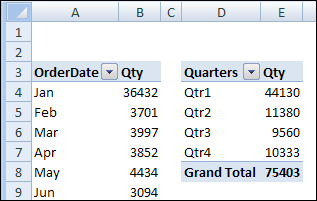
When you change the grouping in one pivot table, the same grouping appears in the other pivot table. For example, change the date grouping in the first pivot table to Months, and the dates in the second pivot table automatically group in Months.

Because you created the two pivot tables from the same source data, by default they use the same pivot cache, which is where the grouping is stored.

However, you might want different grouping in the two pivot tables. For example, you’d like Month grouping in one pivot table, and Quarter grouping in the other.

pivotgroupcache01

Create a Second Pivot Cache

To use different grouping in each pivot table, you’ll need to create a separate pivot cache for each pivot table. Use the following easy method, suggested in the Excel newsgroups by Dave Peterson.

To create a separate pivot cache for the second pivot table:

  1. Cut the second pivot table, and paste it into a new workbook.
  2. Change the grouping of the second pivot table.
  3. Cut the second pivot table from the new workbook, and paste it back into the original workbook.

Now there are two pivot caches in the original workbook, and each pivot table can be grouped independently.

Watch the Video

To see the steps for creating a second pivot cache so you can create separate grouping in the pivot tables, please watch this Excel video tutorial.

________________

Pivot Table Summary Functions: StdDev and StdDevp

Previously, we’ve looked at the pivot table summary functions:  Count, Average, Min and Max and Product. In this article we’ll look at the StdDev and StdDevp summary functions.

StdDev Function and StdDevp Function

Like the STDEV.P and STDEV.S worksheet functions, the StdDev and StdDevp summary functions calculate the standard deviation for the underlying data in the Values area, and is the square root of the variance. Like the variance, standard deviation is a measure of how widely the values vary from the average of the values.

The StdDevp summary function is used when the entire population is used in the calculation. If a sample of the data is used, instead of the entire population, then use the StdDev summary function.

STDEV.P Worksheet Function

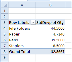
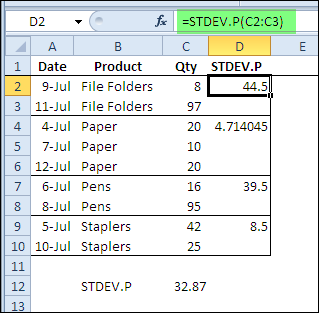
Shown below is the pivot table source data, and the STDEV.P worksheet function is calculating the standard deviation for each product type. There is a large difference between the quantities of file folders sold, and the standard deviation is 44.5. For the paper sales, the difference in quantity is much smaller, and the standard deviation is only 4.71.

pivotstdev00 

Pivot Table StdDevp Summary Function

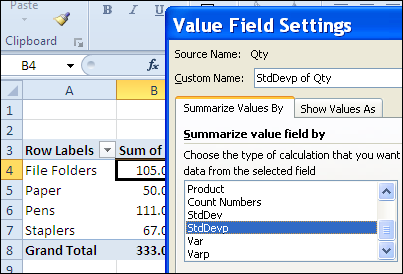
To use the StdDevp summary function, when the Qty field is added to the pivot table, change the summary calculation to StdDevp.

pivotstdev01b 

The standard deviations shown in the pivot table are the same as those that were calculated on the worksheet.

 pivotstdev02  

Note: If the count of items is one, a #DIV/0! error is displayed when using the StdDev summary function, because one is subtracted from the count when calculating the standard deviation.

How the Standard Deviation is calculated

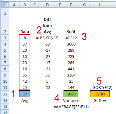
In the standard deviation, each number is compared to the mean of the numbers. If you were to calculate the standard deviation on the worksheet, without the STDEV.P function, here’s how you would do it.

  1. Find the average of the numbers in the pivot table data.
  2. From each number, subtract the average.
  3. Square the calculated difference for each number
  4. Find the average of the squared difference.
  5. Find the square root of the average.

pivotstdev03 

_______________

Pivot Table Summary Functions: Var and Varp

Previously, we’ve looked at the pivot table summary functions:  Count, Average, Min and Max and Product. In this article we’ll look at the Var and Varp summary functions.

Var Function and Varp Function

Like the VAR.P and VAR.S worksheet functions, the Var and Varp summary functions calculate the variance for the underlying data in the Values area, and is the square of the standard deviation. Like the standard deviation, variance is a measure of how widely the values vary from the average of the values.

The VarP summary function is used when the entire population is used in the calculation. If a sample of the data is used, instead of the entire population, then use the Var summary function.

VAR.P Worksheet Function

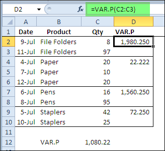
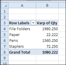
Shown below is the pivot table source data, and the VAR.P worksheet function is calculating the variance for each product type. There is a large difference between the quantities of file folders sold, and the variance is 1980.25. For the paper sales, the difference in quantity is much smaller, and the variance is only 22.22.

pivotvarp00

Pivot Table Varp Summary Function

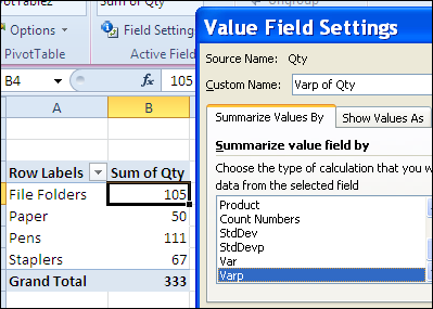
To use the Varp summary function, when the Qty field is added to the pivot table, change the summary calculation to Varp.

pivotvarp01b

The variances shown in the pivot table are the same as those that were calculated on the worksheet.

pivotvarp02  

Note: If the count of items is one, a #DIV/0! error is displayed when using the Var summary function, because one is subtracted from the count when calculating the variance.

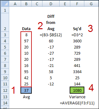
How the Variance is calculated

In the variance, each number is compared to the mean of the numbers. If you were to calculate the variance on the worksheet, without the VAR.P function, here’s how you would do it.

  1. Find the average of the numbers in the pivot table data.
  2. From each number, subtract the average.
  3. Square the calculated difference for each number
  4. Find the average of the squared difference.

pivotvar03

_______________

Pivot Table Summary Functions: Product

In recent blog posts, we’ve looked at the pivot table Count function, the Average function, and the Min and Max functions. In this article we’ll look at the Product function.

Product Summary Function

The Product summary function shows the result of multiplying all the underlying values in the Values area. The result is the same as using the PRODUCT function on the worksheet to calculate the multiplied values.

In all the years that I’ve worked with pivot tables, I’ve never had to use the Product summary function, and can’t imagine a situation where it would be useful. However, you can see how it works, and decide if it would be useful in any of your applications.

PRODUCT Worksheet Function

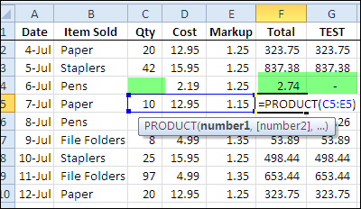
The PRODUCT worksheet function can be useful as a quick way to multiply several values in a worksheet row. For example, in this list of orders, the PRODUCT function multiplies the item quantity, times the cost, times the markup rate, to get the total price for each order.

In column G, you can see the total calculated by using the multiplier operator instead. The only case in which the results are different is where there is a blank cell, such as in row 4. The PRODUCT function treats the blank as a 1, and the multiplier operator treats the blank as a zero.

pivotproduct02 

In this scenario, the PRODUCT worksheet function shows a meaningful result.

PRODUCT Worksheet Function for Columns

However, when you’re using data  as the source for a pivot table, you aren’t multiplying rows, as you would with the PRODUCT worksheet example above. The pivot table will summarize the data from several, or even thousands of rows, so the PRODUCT function isn’t useful, in my experience.

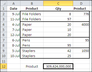
In the screen shot below, you can see the pivot table source data, with the product calculated for each type of item that’s sold, using the PRODUCT worksheet function. Instead of multiplying the values in rows, values in the same column (Qty) are being multiplied.

At the bottom of the source data is the overall PRODUCT calculation.

pivotproduct01

Unlike the previous example, these products are meaningless.

Pivot Table Product Summary Function

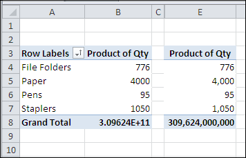
When you use the Product summary function in a pivot table that’s based on the data source shown above, the results are the same meaningless numbers.

The results of the Product function may be very large numbers and default to a Scientific number format. You can format the numbers as Number format, instead of Scientific format.

Note: Excel only stores and calculates with 15 significant digits of precision, so after the 15th character you’ll only see zeros.

 pivotproduct03

_________

Add Pivot Table Wizard in Excel 2007

The Pivot Table Wizard isn’t available on the Ribbon in Excel 2007. To open the Pivot Table Wizard, you can use the keyboard shortcut — Alt + D, P — as described in the article on creating a pivot table from multiple sheets.

Another option is to add the Pivot Table Wizard button to your Quick Access Toolbar (QAT), by following the steps below.

Customize the QAT

To add the Pivot Table Wizard to your QAT, follow these steps:

  • Click on the Customize Quick Access Toolbar button
  • Click More Commands

QATMoreCmd 

  • From the ‘Choose commands from’ drop down list, select ‘Commands Not in the Ribbon’

QATCmdsNot 

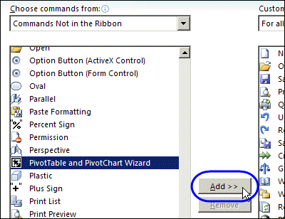
  • In the list of commands, click PivotTable and PivotChart Wizard
  • Click the Add button, then click OK

QATPivotWizard

Open the Pivot Table Wizard

Now that the Pivot Table Wizard button has been added to the QAT, you can click it to open the Pivot Table Wizard.

QATPivotWizard2 

___________

Pivot Table Summary Functions: Max and Min

In recent blog posts, we’ve looked at the pivot table Count function and the Average function. Now we’ll look at two more functions, that are closely related — Min and Max.

Max Summary Function

The Max summary function shows the maximum value from the underlying values in the Values area. The result is the same as using the MAX function on the worksheet to calculate the maximum of the values.

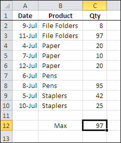
In the screen shot below, you can see the source data for a small pivot table, and the maximum quantity, using the worksheet’s MAX function, is 97.

pivotmax01

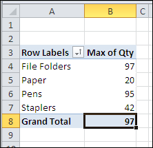
With a pivot table, you can quickly see the maximum for each product that was sold, and the grand total — 97 — which matches the worksheet maximum.

pivotmax02

Min Summary Function

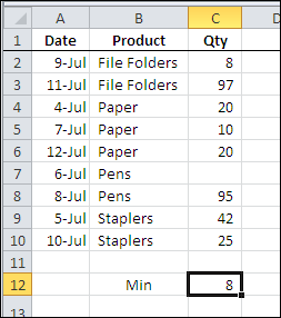
The Min summary function shows the minimum value from the underlying values in the Values area. The result is the same as using the MIN function on the worksheet to calculate the minimum of the values.

In the screen shot below, you can see the source data for a small pivot table, and the minimum quantity, using the worksheet’s MIN function, is 8.

pivotmin01

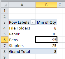
With a pivot table, you can quickly see the minimum for each product that was sold, and the grand total — 8 — which matches the worksheet minimum.

pivotmin02

In both the worksheet and the pivot table, the blank cell is ignored when calculating the minimum amount.

___________


___________

Pivot Table Summary Functions: Average

When you add a numeric data field to the Values area in a pivot table, the summary function defaults to either Sum or Count. You can change that field to use one of the other summary functions, such as Average.

The Average Function

The Average function in a pivot table works like the AVERAGE function on the worksheet to calculate the average (mean) of the values. It totals all the underlying values in the Values area, and divides by the number of values. 

pivottableaverage05 

You can use the Average function to compare amounts, such as order sizes, student grades, and project times, across a large number of instances.

Blanks and Zeros

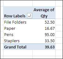
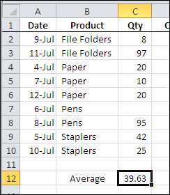
Just as they are on the worksheet, blank cells are ignored when calculating the pivot table averages, but zero cells are included.

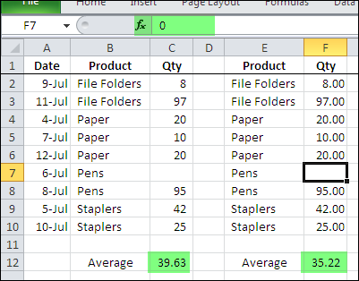
In the data source shown below, cell C7 is blank. That blank cell is not included in either the worksheet average (C12),

pivottableaverage01

or in the pivot table average, shown below.

pivottableaverage05 

Hidden Zeros

If you have formatted the worksheet to hide zero values, remember that those zero values will be included in the averages, even if the cells appear blank.

In the two data sources shown below, the overall average is different. Zeros are hidden on the worksheet, and cell F7 contains a zero. Cell C7 is blank.

pivottableaverage04

If you create pivot tables from these two data sources, the pivot table Average function would include the hidden zeros, just as the worksheet Average does.

Format the Results

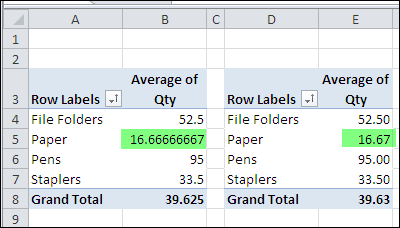
When you use the Average summary function, the results will probably show a strange mixture of decimal places, as shown in the pivot table at the left, in the screen shot below.

pivottableaverage03

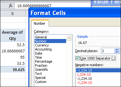
Format the field to have a consistent number of decimal places (as in the pivot table at the right, above), so the numbers are easy to compare.

pivottableaverage02

____________

Pivot Table Summary Functions: Count

When you add a field to a pivot table’s Values area, Count is the default summary function, if the field contains nonnumeric or blank cells. (If the field’s data are all numbers, Sum is the default function.)

The Count function’s name is slightly confusing, because it’s like the COUNTA worksheet function, not the COUNT worksheet function.

The pivot table Count function counts:

  • text
  • numbers
  • errors

Blank cells are not counted.

Watch What You Count

If you’re using the Count function in a pivot table, be careful which field you use for the count. For example, in the pivot table source  data shown below, cell C7, in the Qty column, is blank.

pivottablecount01

if you want to count the order for Pens, and use the Qty field, the blank cell (C7) would not be counted. The number of orders for Pens would show as 1. Instead, you could add the Product field to the Values area, and the Pens orders would show a count of 2.

In the pivot tables shown below, the one on the left uses Qty in the Values field, and the pivot table on the right uses Product in the Values field.

pivottablecount02

__________