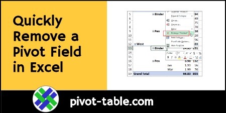
Quickly Remove a Pivot Table Field in Excel

Here’s a quick tip that shows how to remove a pivot table field in Excel. A very short video shows the steps, and there are written steps too, below the video.

Video: Quickly Remove a Pivot Table Field in Excel

Here’s the very short video that shows the simple steps to remove a pivot table field in Excel. The written steps are below the video.

Quickly Remove a Pivot Field

After you create a pivot table, you might want to remove a field from the layout. You don’t need to go to the field list, find that field and remove its check mark, or drag the pivot field out of the Row Labels area in the field list.

To quickly remove a pivot field from the layout, follow these steps:

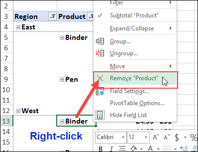
In the pivot field that you want to remove, right-click on the heading cell, or on any item that pivot field
In the pop-up menu that appears, click on Remove [pivot field name]

In this example, I wanted to remove the Product field, so I right-click on the Binder item in that pivot field.

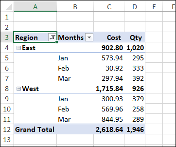
The pivot field is immediately removed from the layout, and the top left cell of the table range is selected.

In the screen shot below, cell A3 is selected.

Macro to Remove Pivot Fields

If you want to remove lots of pivot fields from a pivot table layout, you can use a macro to make the job easier. The macro below removes all the Filter fields from the first pivot table on the active sheet.

There are more macros on my Contextures website – go to the Remove Pivot Fields with Macros page, to find all the macros.

NOTE: If your pivot tables are OLAP-based (using the Data Model), go to the Remove Data Model Pivot Field Macros page instead.

Sub RemoveAllFieldsFilter()
Dim pt As PivotTable
Dim pf As PivotField

Set pt = ActiveSheet.PivotTables(1)

For Each pf In pt.PageFields
  pf.Orientation = xlHidden
Next pf

End Sub

_____________________________