Excel is a great tool for working with a list of data, and calculating sums and counts. Use functions like COUNTIF and COUNTIFS, to get counts based on one or more criteria. But don’t forget about pivot tables, when you need a quick count or sum. With a few clicks, a pivot table will quickly show how many of each item are in a list.
How Many of Each Item?
In this example, 100 people were asked to name their birth month, and the list was entered on an Excel worksheet. The video below shows how to get a count of the number of times each month was mentioned in the survey results. There are written steps below the video.
NOTE: This video shows how to count instances or duplicates of an item. If you need a Distinct Count of items (Unique Count of items), see the steps on my Contextures website.
Video: Count Duplicates With Pivot Table
To see the quick steps to count duplicates, watch this short video. Sarah shows how to count the number of times each month name appears in the list. No formulas are needed!
Prepare the List
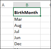
In this example, 100 people were asked to name their birth month, and the list was entered on an Excel worksheet.
A heading, BirthMonth, was added at the top of the list, and formatted as bold text. That formatting helps Excel understand that the top cell is a heading.

Start the Pivot Table
We’ll use a pivot table to count the duplicate entries for each month name. Follow these steps to start the pivot table:
- Select one cell in the list of month names. You can select the heading cell, or any one of the month names.
- Next, click the Insert tab on the Excel Ribbon
- Click the Pivot Table command
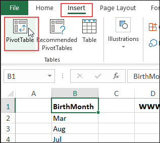
Pivot Table Table or Range
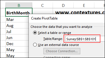
In the Create Pivot Table dialog box, the list’s address should automatically appear in the Table/Range box.
- If the correct range isn’t shown, click in the Table/Range box
- Click on the worksheet, and select the heading cell, and the list of month names
Pivot Table Location
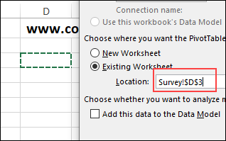
You can choose a location where you want the pivot table to be placed – a new worksheet or an existing worksheet.
- For this pivot table, I’ve selected Existing Worksheet.
If that option is selected, you need to select the sheet and cell where you want the pivot table to start.
- I’ve selected cell D3 on the Survey sheet
Data Model
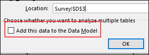
You can choose whether or not to add the data to the workbook’s Data Model.
- If you check that box, you’ll create an OLAP-based pivot table
- If you do not check that box, you’ll create a normal pivot table
These pivot table types have different features and properties, and for this pivot table, it doesn’t matter which pivot table type you create.
I left the box unchecked, to create a normal pivot table
Create the Pivot Table
After you’ve selected the options that you want, click the OK button, to create an empty pivot table on the worksheet.
- The first cell in the pivot table should be selected
- You should see a PivotTable Fields List – usually at the right side of the Excel window.

Add Month Names to Pivot Table
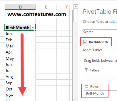
In the PivotTable Field List, there’s only one field name – BirthMonth
- To show a list of months, add a check mark to BirthMonth
- Because the list is text only, the field is automatically added to the Rows area, in Month order
Count the Duplicates
Next, we want the pivot table to show a count of the duplicate month names in the survey results. How many instances are there of each month name?
To show the count:
- In the Pivot Table Field List, drag the checked BirthMonth field down into the Values area
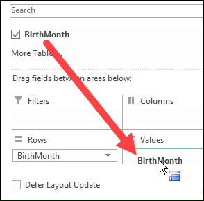
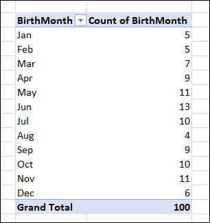
A new column appears in the pivot table, with the heading, “Count of Birth Month”
In that column, the pivot table shows the number of times that each month name appears in the survey results list.
Enhance the Pivot Table
You can leave the pivot table as is, or you can make a few final touches to enhance it.
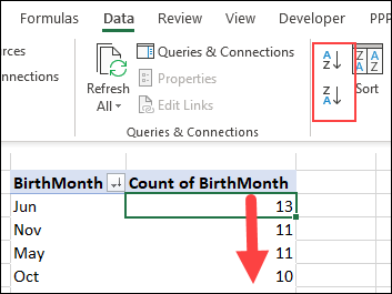
By default, the month names are listed in month order. You might prefer to see the list sorted by the numbers n the count field. To sort by Count:
- Select any number in the Count column
- On the Excel Ribbon, click the Data tab
- In the Sort & Filter group, click the A-Z button (smallest to largest), or the Z-A button (largest to smallest)
The list of months will be sorted based on the numbers in the Count column
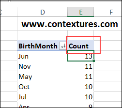
You could also change the heading in the Count column:
- Click on the heading cell – “Count of BirthMonth”
- Type a new heading, e.g. “Count”
- Adjust the column width, to fit the new heading
Get the Sample File
To get the sample file, go to my Contextures website – Count Duplicates With a Pivot Table. The zipped file is in xlsx format, with no macros. You can use the workbook to follow along with the video.
Use Formulas to Count Duplicates in Excel
Instead of using a pivot table, you could use Excel functions to count duplicates.
Go to my Contextures website to see how to use functions like SUMIFS and COUNTIFS, to get a count or a sum, based on one or more criteria.
______________________
Quickly Count Duplicates with Excel Pivot Table

_______________
______________________
