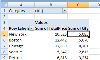
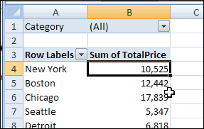
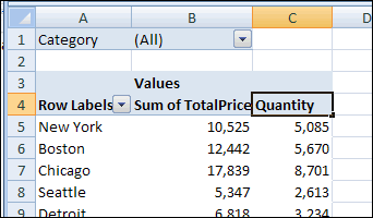
Occasionally, you might need to change a column heading in the pivot table’s source data. For example, you could change a column heading from Qty to Quantity, to make it easier to understand.

However, when you refresh the pivot table after making the changes, the renamed field will disappear from the pivot table layout. In our example, the Qty field is removed from the layout. It isn’t automatically replaced by the Quantity field, even though it’s in the same column heading cell in the source data.

If you change the column headings, you’ll have to add the revised field to the pivot table layout again. If you had number formatting in the old pivot field, you’ll have to reapply the number formatting you had previously applied.
Change Captions Instead
If possible, instead of changing the column headings in the source data, create custom names for the fields in the pivot table instead.
For example, to create a custom name for the Qty field:
- In the pivot table, click on the cell that contains the pivot field name, Qty.
- Type the custom name, Quantity.
- Press the Enter key, to complete the renaming.

_____________________
For more information on Pivot Tables, please see the Pivot Table Tutorials on the Contextures Website.
_________________

Hello,
Any possiblity to change the pivot table column heading to a dynamic name ie. the report change weekly the column Sum of Qty change from Week 1 Sales Qty to Week 2 Sales Qty, can formula apply to C4?
Thanks
Jenny
@Jenny, you can’t use a formula as a pivot table heading. You could use a macro to change the heading text each week, and set it up to run automatically when the workbook opens.
Hi Debra,
I was trying to take your advice above and make the change via vba, but was unsuccessful using several variations of the code below. Any ideas on how to get this to work? Thanks!
Sub test()
i = Worksheets(“Consolidated”).Range(“M1”).Value ‘the data source header cell that changes
Worksheets(“Summary”).PivotTables(1) _
.PivotFields(“Category”).SourceName = i
End Sub
Hi,
Having some wizz pivot masters around here, and also being beyond basic excel myself, I need some help on the following.
In the build up of the Pivot table I had a date field on the left comming from a source.
Then, one of these dates we “abused” and overwrote as “PENDING” in the pivot……now moving along in time this date is becoming an actual date I want to use in the pivot……..so, how do I reverse it back to actually become a date again?
We tried lots of stuff, but couldn’t work it out…..hope another pivot wizz is reading this (or even pro wizzes making excel) to help solve my issue.
Thanks!
Johnny
I have the formula “=TODAY()-6” as my source-data (column) header. Every day I refresh, I have to reformat my Pivot Table. Why can’t the Pivot Table rely on $R$3 rather than on $R$3’s contents?
It would be wonderful to have the pivot table update on refresh to reflect changed labels.