With a pivot table, it’s easy to show a total Sum or Count, or other quick summaries. You can also use the Show Values As options, to show each number compared to other items in the pivot table. There are several options, such as running total, % of Grand Total, and Difference From other amounts. In this example, we’ll show the units sold for each item, as a % of parent total (% of subtotal).
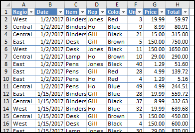
Excel Table with Product Sales Data
In this example, there is a table with product sales. It has been formatted as a named Excel table, with the name tblSalesData.
Show Sum of Units in Pivot Table
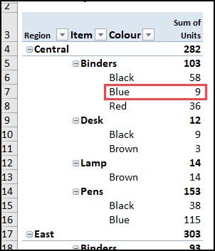
On a different worksheet in the workbook, a pivot table is based on that Excel table. The Region, Item and Colour fields are in the Row area, and Units is in the Values area.
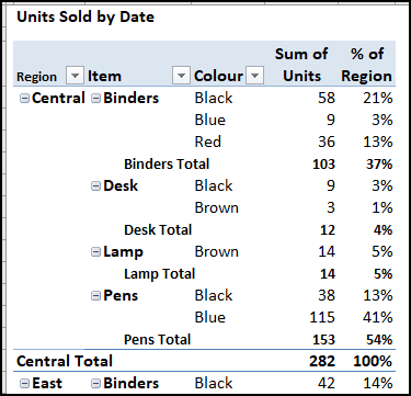
The pivot table shows the Sum of Units for each Region/Item/Colour combination. For example, 9 blue binders were sold in the Central region.
Add Another Value
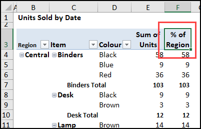
To see how each amount contributes to the overall region sales, we’ll add a new column of values:
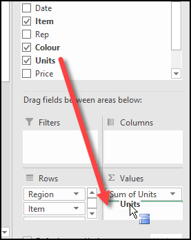
- In the Pivot Table Field List, drag another copy of the Units field to the Values area, below the first copy
- In the pivot table, change the heading of the new column to % of Region. That makes it easier to understand the data.
Show Values As % of Parent Total
Next, change the Show Values As setting, to see each total compared to the region’s total.
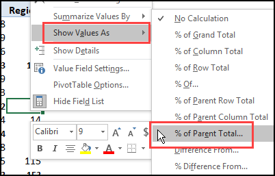
- In the % of Region column, right-click on one of the numbers
- Point to Show Values As, then click % of Parent Total…
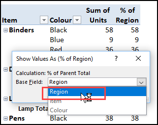
- In the dialog box that appears, select Region as the Base Field – we want to see each value as a percent of the Region’s total.
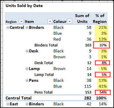
The % of Region column changes, to show the percent of the Region’s total.
NOTE: The numbers are formatted as Percentage, with 0 decimals.
% of Region Totals
With the Show Values As % of Parent Total option, you select a specific field to use as the Base for comparison. We chose Region, so the other values are compared to the Region totals:
- The percentages for the colours are highlighted in yellow. They show each item/colour percentage of the total units for the Central region. For example, the 9 blue binders make up 3% of the total units in the Central region.
- The percentages for each product (Item) are outlined in red. They show each product’s percentage of the total units for the Central region. For example, the 103 binders make up 37% of the total units in the Central region.
- The percentage for the Base field (region) is outlined with a blue oval. The base field will always be 100%, because its total is being compared to itself.
Get the Excel Workbook
To get the free Excel workbook for the Show Values As % of Parent Total example, go to the Pivot Table Show Values As page on my Contextures website.
You’ll also find examples for the other Show Values As options, such as Running Total, Rank, Difference From, and % of Grand Total.
_____________


Big Help, Thanks…
Hi,
when I work with my pivot table except the sum, average and count all the other functions in the calculation field doesn’t work. I get a o or div/0error. could you please advise me?
Hello,
1. Why “% of parent row total” compares each item to column total and “% of parent column total” compares each item to row total? (I tested it and it is so)
2. What does “parent” mean in a pivot table?