Show Percent Difference in Pivot Table Amounts

With one of the built-in custom calculations in a pivot table, you can quickly show the percent difference between two amounts. In this example, forecast amounts have been entered for each product, for each month. When they become available, the actual amounts are entered in the workbook.

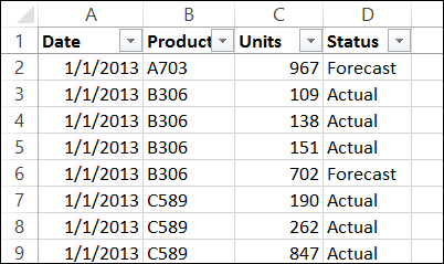
In the next screen shot, you can see how the data is set up. There is a Status column, and “Forecast” or “Actual” is entered there. All the Units quantities are entered in column C. With this setup, we can easily compare the Forecast and Actual amounts.

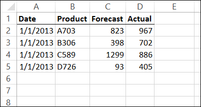
If your data has Forecast and Actual as column headings, and the amounts in separate columns, you won’t be able to use a custom calculation to show the differences. A pivot table custom calculation can only calculate on items within the same pivot field.

Create a Pivot Table

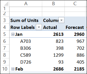
Based on the data in the first screen shot, a pivot table is created. It has the following fields in its layout:

• Rows – Date (grouped by Month), and Product
• Columns – Status
• Values – Units

Grand Totals for Rows have been turned off.

Calculate the Percent Difference

To see the percent difference between the Forecast and the Actual units, you can use a custom calculation.

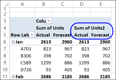
• Add another copy of the Units field to the Values area, where it will become Sum of Units2.
  • 
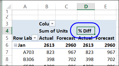
• Select a cell that contains the Sum of Units2 label, and then type a more descriptive name, for example, % Diff.
  • 
• Right-click one of the % Diff cells in the Values area, and click Value Field Settings.
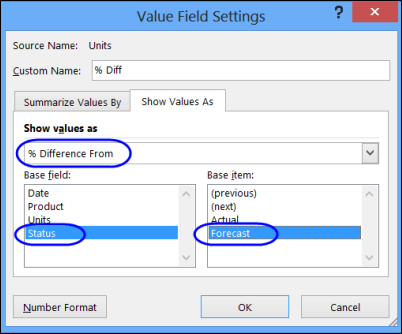
• Click the Show Values As tab, and from the drop-down list for Show Values As, select % Difference From.
• You want to compare the Status field values, so for the Base field, select Status.
• The Actual values will be compared to the Forecast values, so for the Base item, select Forecast.
  • 
• To reduce the number of decimal places, click the Number Format button, and format with Percentage, and the number of decimal places you want.
• Click OK twice, to close the dialog boxes.
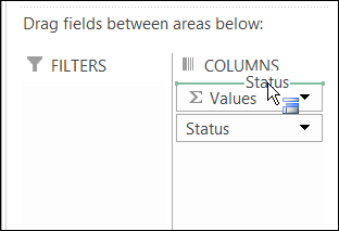
• In the PivotTable Field List, move the Status field below the ∑ Values field in the Column Labels area.
  • 

This changes the order of the columns, so the Units are together, and the % Diff columns are together.

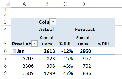
The Forecast column is empty in the % Diff field, because it won’t be compared to itself. The Actual column shows the % Difference From calculation from the forecast in units sold, for each product for each month.

_________________________