By default, the Pivot Table shows only the items for which there is data. In the example shown in this video, not all colours were sold to each customer. You may wish to see all the items for each customer, even those items with no data.
Comparing Product Sales
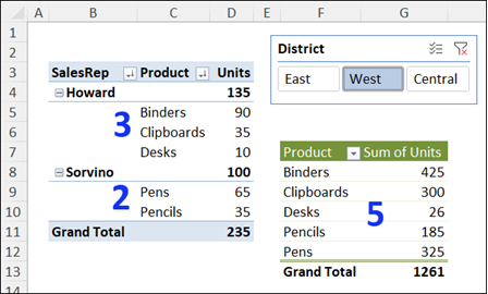
By default, an Excel Pivot Table shows only the items for which there is data. For example, in the screen shot below:
- Company has 5 types of products
- Sales rep Howard sold 3 types of products in the West district
- Sales rep Sorvino sold 2 types of products in the West district
It’s not easy to see, at a glance, which products are missing from each sales rep’s summary.
Frequent Layout Changes
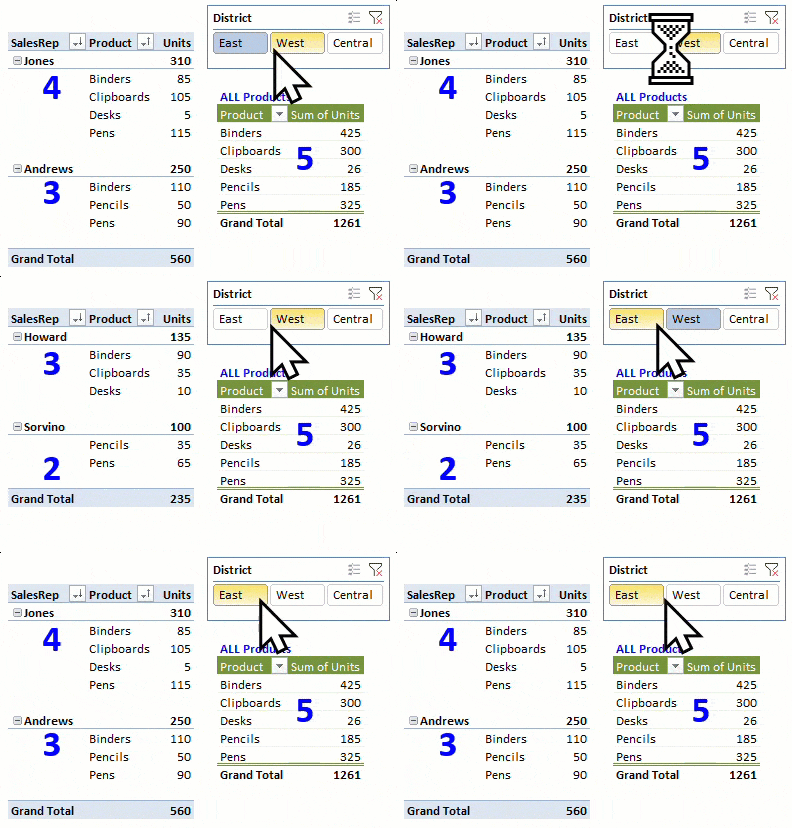
Each time I use the pivot table Slicer to select a District, the pivot table layout changes. Depending on the District and Sales Reps, there is a different number of product types listed.
It would be easier to spot the differences if all 5 products always showed, no matter what district and sales reps are showing in the pivot table layout.
Video: Show Missing Pivot Items
To make it easier to compare product sales between the sales reps, you can change a pivot table setting.
In this short video, I show the simple steps to follow, so all the pivot items show, even if there is no sales data for that item.
When you change this setting, the pivot table layout stays consistent, with all 5 product types showing. That makes it easier to spot what’s missing!
Other Fixes for Missing Data
In some pivot tables, there might be other reasons that some data is missing, and pivot items don’t appear in the pivot table layout.
Source Data: Check the pivot table’s source data settings, to make sure it includes all of the rows and columns. I’ve seen many workbooks where a new column was added to the right of the source data, and that new column wasn’t automatically included in the pivot table source range. For tips on fixing that problem, go to the Pivot Table Source Data page on my Contextures site.
Filters: If there are filters applied in the pivot table, that could prevent some items from appearing. Check the pivot field headings, to see if there are any filter icons. If you find any, point to each filter icon, to see a pop-up tool tip, with details on that filter.
Filter Settings: Pivot table manual filters (checklists) can be set to not show new items that were added to the data, after you applied that filter. The short video below shows how you can adjust that setting, so new items WILL appear in those manual filters.
Get the Sample File
To get the Excel sample file, to follow along with the video, go to the Pivot Table Field Settings page on my Contextures site.
In the Download section, get the Missing Items file, with stationery sales data. The zipped file is in xlsx format, and does not contain any macros.
More Pivot Table Tips
Clear Old Items in Pivot Table
Count Duplicates with Pivot Table
________________
Show All Pivot Table Items To Compare Sales Easily-No Data
________________


