You probably use a few shortcuts when you work with Excel pivot tables. But do you use this pivot table double-click trick, to see the pivot field settings dialog box?
Field Settings Shortcut
Here are the steps for the pivot table field settings shortcut:
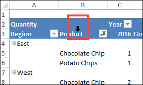
- With your mouse, point to the outer border of a pivot table row or column heading
- When you see the black arrow, double-click, to open the Field Settings dialog box.
Shortcut to Hide Pivot Fields
There are more pivot table field shortcuts too. This very short video that shows the mouse shortcut for hiding pivot fields.
- Right-click on an item in the pivot field. In the video, a cell in the Product field was right-clicked.
- Click Remove [field name]
More Pivot Table Shortcuts
For even more pivot table shortcuts, go to my Contextures website. There’s a list of shortcuts, and an Excel workbook that you can download.
For example, here’s a shortcut for creating a pivot table calculated field
- Select any field in the Values area
- Press Chtr + Shift + = (equal sign)
- That opens the Calculated Field dialog box, where you can create the calculated field

Shortcut to Group Pivot Items
Here’s another quick shortcut for pivot tables – use it to group a few text pivot items.
- In the pivot table, select the pivot items that you want to group
- Tip: For non-adjacent items, select the first cell, then press the Ctrl key while selecting additional pivot item cells
- Press Alt + Shift + Right Arrow
- The selected items are grouped, and a new field might be created, like Category2 in the screen shot below.
See more pivot table grouping tips on my Contextures site.

More Field Setting Tips
For more field setting tips, macros, videos and sample files, go to the Excel Pivot Table Field Settings page on my Contextures site.
___________________________________
Excel Pivot Table Shortcut for Field Settings
___________________________________


