After you create a pivot chart, you can change the number format for axis labels. This video shows the steps. Change just the pivot chart, or change both the pivot table and pivot chart number format.
Video: Change Pivot Chart Number Format
At first, a pivot chart’s axis labels use the same number format as the pivot table it’s based on. This video shows the steps for changing that axis label number format.
Video Timeline:
- 0:00 Introduction
- 0:22 Create a Pivot Chart
- 0:41 Change Number Format
- 1:16 Number Format Chart Only
- 1:35 Number Options
- 1:53 Custom Number Format
- 2:36 Get the Workbook
Use Different Number format in Pivot Chart
Recently, I wrote about the steps for changing the number format in a pivot chart, so it’s different from the pivot table number format.
The video also shows how you can change the number format for both the pivot table and pivot chart, at the same time.
Here are the steps to follow:
- In the pivot table, right-click on a cell in the value field. In this example, the Cases field is used.
- In the popup menu, click Value Field Settings, and then click the Number Format button
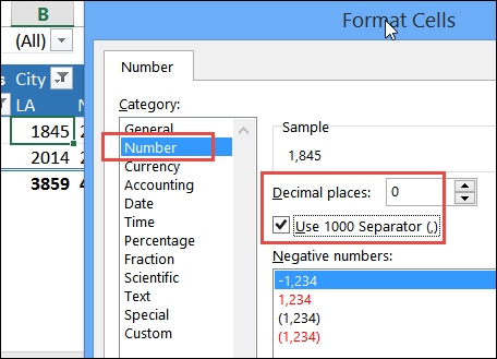
- In the Format Cells dialog box, select the formatting that you want.
- In the screen shot below, the Number category is selected, with decimal places set to 0
- A check mark was added to “Use 1000 Separator”
- Click OK, twice, to close the dialog boxes
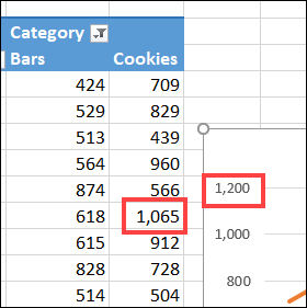
The number format change is applied to both the pivot table and the pivot chart.
Get the Excel Workbook
For more details on pivot chart numbering, and to get the sample workbook, go to the Pivot Chart Number Formatting page on my Contextures site.
The sample file also has a pivot chart formatting macro, that makes it quicker to format several pivot charts at once, and there are sample pivot charts for testing.
_______________________
Change Pivot Chart Number Format Video
______________________


