Show Sales Amounts as Data Bars in Excel Pivot Table

Most pivot tables show numbers, so you can see a detailed summary of the source data. To add a visual element to the pivot table, add data bars that are similar to a bar chart. This works well in a simple pivot table, with only one or two columns of data.

Data Bars in Pivot Table

This short video shows the steps for setting up a pivot table with data bars, and there are written steps below the video.

To get the workbook that I used in the video, go to the Pivot Table Conditional Formatting page on my Contextures site.

Video Timeline:

0:00 Introduction
0:12 Create a Pivot Table
0:47 Add Fields
1:00 Filter and Format
1:37 Add Data Bars
2:27 Format the Data Bars
3:02 Data Bar Problem
4:30 Get the Workbook

Simple Pivot Table

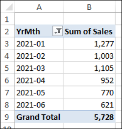
For this example, there is a simple pivot table with, with only 2 fields in the layout:

YrMth field in Rows area, filtered to show Jan-June
Sales in Values area, formatted as number, zero decimals, 1000 separator

Add Pivot Table Data Bars

To create data bars in a pivot table, you’ll use conditional formatting. Later, there are special settings that you need to apply, so the formatting will update correctly.

Here’s the quickest way to add data bars:

In the pivot table, select the sales amounts in cells B3:B8
- Don’t select the Total cell
On the Ribbon’s Home tab, click Conditional Formatting
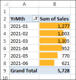
Click Data Bars, and click one of the Data Bar styles

Data Bars appear in the sales amount cells, along with the number.

There’s a small problem with this quick method though, and you’ll see the quick fix in a minute.

Hide the Data Bar Numbers

After you add data bars, it can be hard to read the numbers that are also in the cells.

I like to remove numbers from the data bar cells, then add another column to show the numbers separately.

Here’s how to hide the numbers in the data bar cells:

Select any cell in the pivot table
On the Ribbon’s Home tab, click Conditional Formatting
Click Manage Rules
In the list of rules, select the Data Bar rule
Click Edit Rule, to open the Edit Formatting Rule window.
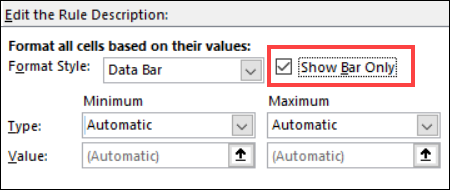
In the Edit the Rule Description section, add a check mark to Show Bar Only
Click OK twice, to close the windows.

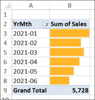
Now the numbers are hidden in the data bar cells.

Conditional Formatting Problem

As I mentioned, there’s a little problem with the quick method of adding data bars, or any other conditional formatting, in a pivot table.

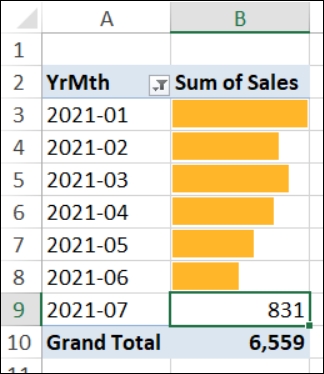
Here’s what happens when I change the filter, and show the July sales – there’s no data bar for that month.

The conditional formatting was only applied to cells B3:B8.

Fix the Conditional Formatting

Fortunately, there’s a quick fix for that problem!

Go back to the Conditional Formatting Rules Manager, to edit the Data Bar rule.
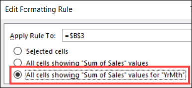
In the Apply Rule To section, select the 3rd option, All Cells Showing “Sum of Sales” Values for “YrMth”
Click OK twice, to close the windows.

Note: The 2nd option would include the Total cell, but the 3rd option doesn’t

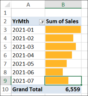
Now the July cell has a data bar. Also, if the filter changes later, any other months will show data bars.

Show Numbers Separately

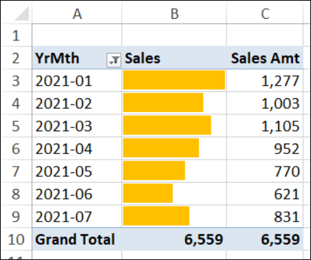
For some pivot table, it might be fine to just show the data bars. But, if you want to see the numbers too, put them in a separate column.

First, select any cell in the pivot table
Then, in the PivotTable Fields list, drag another copy of the Sales field to the pivot table Values area
Next, format those values as Number, zero decimal places, 1000 separator
Optional: Change the headings to “Sales ” (with a space at the end), and “Sales Amt”