If you create two or more pivot tables from the same source data (pivot cache), you can connect them to the same Excel Slicers. That will make it easy to filter all the connected pivot tables at the same time.
Video: Connect Slicers to Multiple Pivot Tables
First, this video shows the easy steps for creating Excel Slicers, based on one pivot table. Next, see how to connect another pivot table to the same Slicers. The written instructions are below the video.
Video Timeline:
- 00:00 Introduction
- 00:22 Two Pivot Tables
- 00:58 Add Slicers
- 02:55 Connect Another Pivot Table
- 04:29 Get More Information
Insert the Slicers
It’s easy to add an Excel Slicer for a pivot table:
- Select any cell in the pivot table.
- On the Analyze tab of the Excel Ribbon, click Insert Slicer.
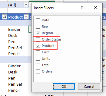
- Next, add check marks to the fields you want as Slicers
- Finally, click OK
Adjust the Slicers
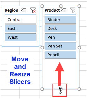
After the Slicers are added to the worksheet, you can move and resize them, so they’re not covering up the pivot tables.
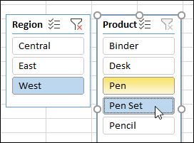
Then, click on an item in the Slicer, to filter the connected pivot table.
Connect Slicer to Another Pivot Table
Next, follow these steps to connect the Excel Slicers to the second pivot table:
- Select a cell in the second pivot table
- On the Excel Ribbon’s Analyze tab, in the Filter group, click Filter Connection

- In the Filter Connections window, add a check mark to each Slicer that you want the pivot table to connect to

Filter Both Pivot Tables
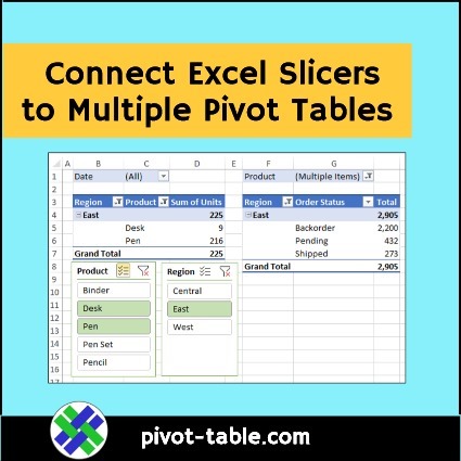
After both pivot tables are connected to the Slicer, when you select an item in a slicer, both pivot tables will be filtered.
For example, in the screen shot below, both pivot tables are showing East region sales, for Desk and Pen orders.

Get the Pivot Table Slicers Workbook
To get the free Excel workbook for this video, go to the Pivot Table Slicers page on my Contextures website. The zipped file is in xlsx format, and does not contain macros.
_____________________
Connect Excel Slicers to Multiple Pivot Tables
____________________


