Pivot Table Value Errors

If there are errors in an Excel table, you might see those errors when you summarize that data in a pivot table. See which Summary Functions show those errors, and which ones don’t (most of the time!)

Excel Table with Errors

In the screen shot below, there is a small Excel table, with several errors and missing or invalid data.

There is text in cell C4, so the formula in E4 has a #VALUE! error, instead of a numeric result
There are three #DIV/0 errors, because Excel can’t divide by zero
There is a blank cell (E7), where a formula has been deleted
Two cells (C4 and E9) contain text, instead of the numbers that should be in those columns

You can download this sample file from the Pivot Table Summary Functions page on my Contextures website.

Create a Pivot Table

To see how Excel handles these errors, I created a new pivot table, based on that table.

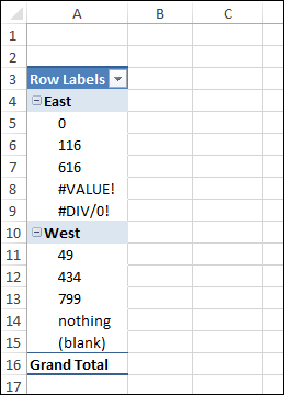
When I added the Region and Total fields, Excel put both fields into the Row area, with the errors showing as items for the Total field. (Excel put Total in the Rows area because it has non-numeric data.)

Move the Total Field

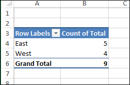
To fix that problem, I moved the Total field to the Values area. Because of its non-numeric values, Excel automatically used the Count summary function for the data.

The error values have disappeared from the pivot table, and the counts for each Region are showing correctly.

Change to Sum Function

In the pivot table, I’d like a sum of the Total amounts – not a count of them.

To change the Summary Function,

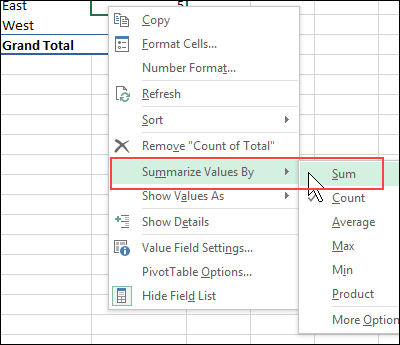
Right-click on one of the numbers in the Count of Total column
Click Summarize Values by, and click Sum

Errors with Sum Function

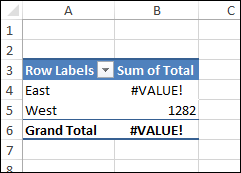
As soon as the function changes to Sum, errors appear in the pivot table, for the East region, and in the Grand Total.

There are special error rules for the Count and Count Numbers Summary functions. For all other Summary Functions, these are the rules if the source field contains error values:

the first error encountered in the source data is displayed in the pivot table
the total is not calculated – it shows the first error from the source data.

In the data’s Total field, #VALUE! is the first error listed for the East region, so that error appears in the pivot table.

Errors with Count and CountNumbers

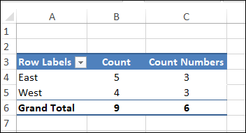
The Count and CountNumbers Summary Functions don’t show error values in the Item summaries. – these functions count the errors, or ignore them.

Count Numbers: Blank cells, errors, and text are not counted.
Count: Text, numbers and errors are counted. Blank cells are not counted.

In this screen shot, you can see the different calculations, with a Grand Total of 9 in the Count column, and only 6 in the Count Numbers column.

Errors in Totals and Subtotals

Even though the Count and Count Numbers functions don’t show errors in the item totals, you will see error values in their Subtotals and Grand Totals, if both of these conditions are met:

Oher summary functions are included in the pivot table, and those fields contain errors in the data
There are error values in the fields used for the Count and Count Number columns

Grand Total Example

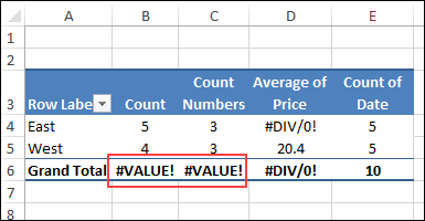
For example, in the screen shot below, two more Values have been added to the pivot table:

Average for the Price field (Price field contains a #DIV/0! error)
Count of the Date field (Date field has no error values)

Because of this change to the pivot table, the Count and Count Numbers columns show error values in their Grand Totals. The item totals in those columns are not affected, and continue to show numbers.

The Count of Date column shows a number in its Grand Total. It does not have any errors in its source data, so it isn’t affected by the error values in the other fields.

Get the Sample File