When you build a pivot table, Excel automatically creates a numbered name for it, such as PivotTable1. You can leave that automatic name as it is, or change an Excel pivot table name to something more meaningful, such as “SalesPivot”.
Create a Pivot Table
While you’re building an Excel pivot table, you don’t have an option to set a name for your pivot table. Excel will create a name, and it’s easy to change the pivot table name at any time.
Watch this video to see the steps for creating a pivot table, using the Recommended Pivot Tables command. You can see written instructions and screen shots on my Contextures website.
See the Pivot Table Name
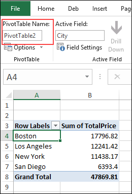
When a pivot table cell is selected, you can see the pivot table’s name at the left end of the Analyze tab on the Excel Ribbon.
Change the Pivot Table Name
You can use that pivot table name box to make a quick change to the pivot table name:
- Click in the PivotTable Name box
- Type a new name, or make a change to the existing name
- Click anywhere outside of the name box, to complete the name change (you don’t have to press Enter)
See the Changed Name
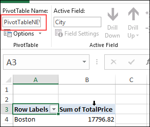
In the screen shot below, I changed the name to “PivotTableNEW”. The name box is small though, and the end of the name is not visible.
NOTE: There’s no setting that lets you increase the size of the pivot table name box on the Analyze tab.
Pivot Table Options
Another place to see the pivot table name is in the PivotTable Options dialog box.
To open the PivotTable Options window:
- Right-click on any cell in the pivot table
- In the right-click menu, click PivotTable Options.

Name Box in Pivot Table Options
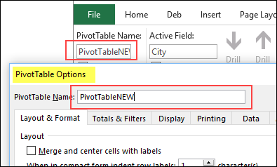
At the top of the PivotTable Options window, there is a box that shows the current name of the selected pivot table.
PivotTable Options name box is bigger than the one on the Analyze tab, so you might want to make changes here, except for very short names.
In the screen shot below, you can see a comparison of the box sizes. The Analyze tab box is about 1″ wide, and the PivotTable Options box is about 2.5″ wide
Pivot Table Name Rules
Although the naming rules for other items, such as macros, or worksheets, are somewhat strict, the pivot table names are quite flexible.
Here are the limits on the number of characters in a valid pivot table name:
- Minimum number of characters: 1
- Maximum number of characters: 256
No Duplicates on Sheet
There is also a restriction on duplicate names:
- You cannot give a pivot table the same name as another pivot table on the same worksheet.
If you try to use a duplicate name, Excel shows an error message, and does not change the existing name.
- “A PivotTable report with that name already exists on the destination sheet.”

Non-Alpha-Numeric Characters
For Excel worksheets, some characters, such as question marks and colons, are not allowed. So far, I haven’t found any characters that are restricted for pivot table names. You can even name a pivot table with a question mark, or one space character!
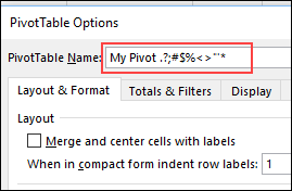
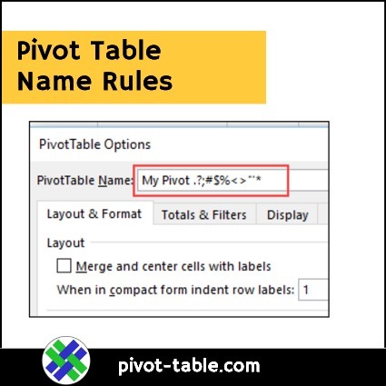
For example of what’s allowed, I changed a pivot table to this strange mix of characters, with no problems.
- My Pivot .?;#$%<>”‘*
NOTE: Even though those odd characters are allowed in pivot table names, I recommend using alphanumeric characters only, to avoid problems when creating macros that refer to pivot tables by name.
More Pivot Table Tips
For more details on building a pivot table, go to the Create a Pivot Table page on my Contextures site. Download the sample file there, and build a pivot table from the data, and then change its name.
For more information on pivot table options, go to the Pivot Table Option Settings page on my Contextures website.
_______________________________
Excel Pivot Table Name Rules
_______________________________


