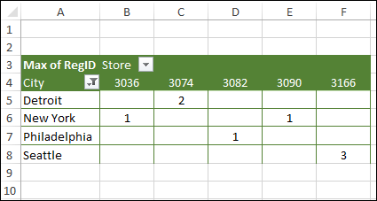
Show Numbers as Text in Pivot Table Values

In an Excel pivot table, you can add text fields to the Row and Column areas, and in the Report Filters. However, pivot table Values area will only show numbers, so if you add a text field there, Excel shows a count of those text items. The technique shown below lets you show number fields as text Values, so you can display the names (East, West), instead of ID numbers (1, 2), for a small group of items.

Video: Show Pivot Table Values as Text

This technique uses a custom number format, applied with conditional formatting. For a few items, you can create the conditional formatting rules manually.

Watch this video to see the steps for setting up 3 ID numbers to show as names. You can learn more about Pivot Table conditional formatting on my Contextures website.

Custom Number Format

In this technique, a numeric field (RegID) is added to the pivot table Values area, and summarized by the Max function.

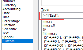
Next, custom number formats are applied as conditional formatting rules. For example, this rule displays “East” if the cell contains the number 1.

[=1]”East”;;

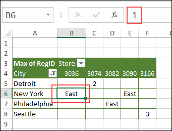
With that rule applied, you can see the number 1 in the Formula Bar, but the pivot table Values cell show the text, “East”.

Use a Macro

If you have several numbers, and want to create conditional formatting rules for them, it will be quicker to use a macro to set up the rules.

Thank you to Prof. Lee Townsend, who contributed the macro shown below. The code has an array of 3 numbers to change to region names. You can change those numbers and names, or add more, if necessary, to match your pivot table items.

For example, if you have 5 regions, change the regionNames and regionNumbers lines, to include all 5 items.

regionNames = _
  Array("East", "Central", "West", "North", "South")
regionNumbers = Array(1, 2, 3, 4, 5)

Macro to Set Rules

Here is the macro to set the conditional formatting rules with the custom number format. Add this code to a regular code module in your workbook. Then, select a cell in the pivot table, and run the macro.

Option Explicit
Option Base 1

Sub ApplyCFArrays()
'by Prof. Lee Townsend
'downloaded from contextures.com
'select a pivot table cell
'then run this macro

Dim CFRange As String
Dim pvt As PivotTable
Dim CellOne As String
Dim colonLocation As Integer
Dim iLoop As Long
Dim regionNames As Variant
Dim regionNumbers As Variant
Dim currentName As String
Dim quote As String
regionNames = _
  Array("East", "Central", "West")
regionNumbers = Array(1, 2, 3)
  
quote = Chr(34)

On Error Resume Next
Set pvt = ActiveCell.PivotTable
On Error GoTo 0
If pvt Is Nothing Then
  MsgBox "Please select a pivot table" _
     & vbCrLf _
     & "cell and try again"
  Exit Sub
End If

'find the location of the top left of
'the pivot table's DataBodyRange
CFRange = pvt.DataBodyRange.Address
colonLocation = InStr(CFRange, ":")
CellOne = Left(CFRange, colonLocation - 1)
CellOne = Replace(CellOne, "$", "")
  
'Start the conditional format rule
CellOne = "=" & CellOne & "="

'Set up the arrays
' https://stackoverflow.com/questions
'   /39509796/is-there-a-way-to
'   -assign-values-to-an-array
'   -in-vba-using-a-single-line
  ReDim Preserve regionNames(1 _
    To UBound(regionNames) + 1)
  ReDim Preserve regionNumbers(1 _
    To UBound(regionNumbers) + 1)
  
'Set up the loop
For iLoop = 1 To 3
  currentName = "[=" _
    & regionNumbers(iLoop) & "]" _
        & quote & regionNames(iLoop) _
        & quote & ";;"
  
  With Range(CFRange).FormatConditions _
    .Add(Type:=xlExpression, _
      Formula1:=CellOne _
      & regionNumbers(iLoop))
    .NumberFormat = currentName
  End With
Next iLoop

End Sub

Get the Sample File

To download the sample file, go to the Pivot Table Text Values page on my Contextures website. There are 2 files available – one has the macro, and the other file does not have any macros.

If you download the file with macros, be sure to enable macros, after you unzip the file and open it.

___________________________