Pivot tables are a quick way to summarize your data, and they have another advantage too. After you build the pivot table, it’s easy to change pivot table layout, to get a different type of summary. Watch the video below, and get the free workbook.
How to Change Pivot Table Layout Video
See how to create an instant pivot table, then make simple changes to its layout. Written instructions are below the video.
Multiple Fields in Values Area
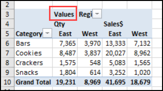
If you have 2 or more fields in the Values area of the pivot table, Excel automatically creates a new field in the layout, called “Values”.
You can see that field on the worksheet, near the top left of the pivot table.
PivotTable Field List
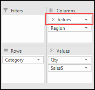
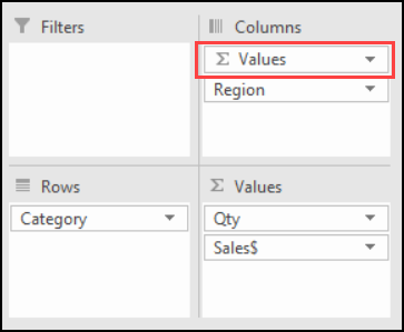
You can also see the Values field in the PivotTable Field List. It shows the Sigma symbol, just like the AutoCorrect command on the Excel Ribbon.
Read more about that Values field on my website. There is a free workbook there too, that you can use for testing.
Pivot Table With One Value Field
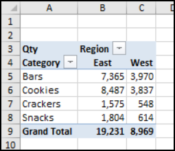
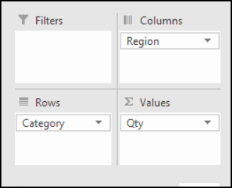
To see how the Values field is added automatically, here is the pivot table with only one field in the Values area. In the screen shot below:
- Category is in the Rows area
- Region is in the Columns Area
- Quantity (Qty) is in the Values area of the pivot table.
Only those 3 fields appear in the PivotTable Field List.
Add Another Value Field
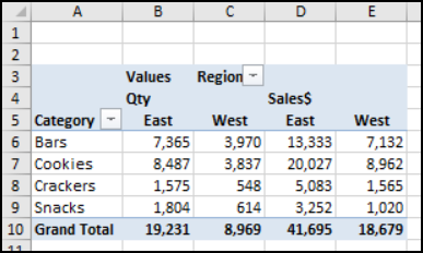
Next, I’ll add the SalesPrice (Sales$) field to the Values area of the pivot table. Excel automatically created the Values field, and its name appears in cell B3.
Now the pivot table shows the Quantity for each region, and then the Sales total for each region.
By default, Excel puts that “Values” field in the Columns area of the pivot table, above the other column fields. Here’s where it appears in the PivotTable Field List.
Change Pivot Table Layout
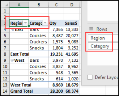
To quickly see a different view of the data, you could move the Row or Column fields. Here is the same pivot table with Region in the Rows area, before the Category field.
Move the Values Field
Another quick way to change pivot table layout is to move the Values field. It can be in the Rows area or the Columns area, but not the Filters area or Values area.
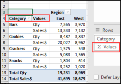
In the screen shot below, I’ve moved Region back to the Values area, and put the Values field in the Rows area, below Category.
This makes a taller, narrower pivot table, so it’s a good layout if you have to print it out in portrait mode.
Experiment With the Pivot Table Layout
Whenever you create a pivot table, take a few minutes to what happens when you change pivot table layout. When you experiment, you might find a new layout that your really like! But don’t worry – if you prefer the original pivot table layout, just Undo, or drag the fields back where they started. Read more about pivot table layout changes on my Contextures website.
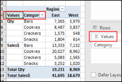
If you have multiple Values fields, remember that you can move the Values field, just like you can move the Row and Column fields.
For example, here is another layout of the same pivot table, with the Values field before the Category field in the Rows area.
Free Pivot Table Tool
If you’re working with pivot tables, I’ve got a free tool that you can use —Pivot Power Free (PP Free). Use it to quickly change Sum to Count, format numbers, and a few other handy things.
Note: If you have a copy of my Pivot Power Premium (PPP) tool, you won’t need this free version. The premium version has all the same tools, and many more.
______________

One thought on “Quickly Change Pivot Table Layout”