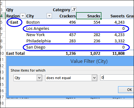
If you create a calculated item, extra items might appear in the pivot table, with zero amounts in some rows. In the example shown below, a calculated item was created in the Category field. Because of that, all the cities are listed under each region, instead of just the region in which they are located.
Los Angeles and San Diego are not in the East, so their sales in that region show up as zero. It makes the pivot table look messy and confusing!
To hide these zero items, use a Values filter. For example, in this screen shot, the City field is being filtered, to hide any rows where the quantity is zero. You can see the step-by-step instructions in the video below.

Video: Hide Zero Items and Allow Multiple Filters
There are 3 types of filters available in a pivot table — Values, Labels and Manual. If you want to apply more than one type of filter, change a setting in the pivot table options, to allow that.
Watch this video to see how to create a calculated item, hide the zero value rows, and allow multiple filter types.
More Pivot Table Tutorials
Calculated Items vs Calculated Fields
____________
