In a pivot table, you can show totals for each calendar year or month:
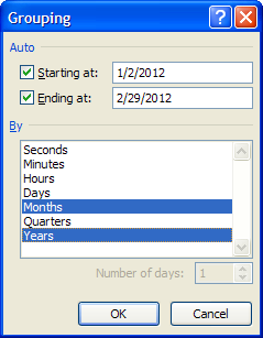
- either group the dates,
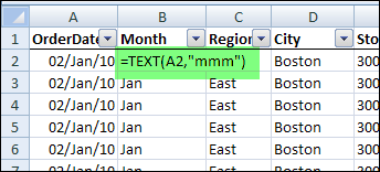
- or calculate the year and month in the source data.
Group By Fiscal Year and Month
There isn’t a built in way to group by fiscal year and month, but you can add formulas in the source data to calculate those.
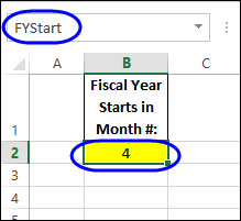
I’ve created a sample file that shows how you can do this, and there is a named cell – FYStart – where you enter the start month of the fiscal year.
Calculate the Fiscal Year
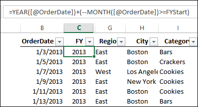
Then, in the source data, there is a Fiscal Year column that checks that cell, to calculate the fiscal year.
=YEAR([@OrderDate])+(–MONTH([@OrderDate])>=FYStart)
- The YEAR function returns the year for the order date.
- If the order MONTH is greater than or equal to the fiscal year start month, 1 is added to the order year. If not, a zero is added.
(The two minus signs are a double negative, and they convert the TRUE result to a 1)
Calculate the Fiscal Month
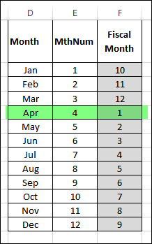
For the Fiscal Months, there is a lookup table, with a list of all the months, and their calendar month number and fiscal month number. In this example, the fiscal year starts in April.
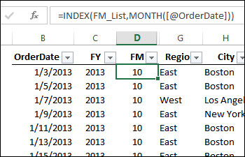
In the source data a Fiscal month formula looks up the fiscal month, based on the order month.
Total by Fiscal Year and Month
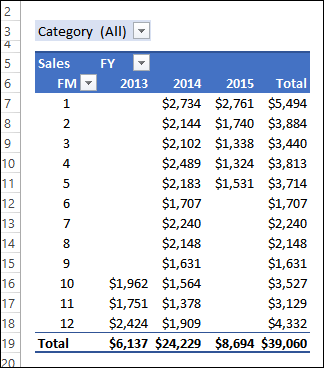
After those fields have been added to the source data, you can put them into the pivot table, to show totals for fiscal year and month.
In the screen shot below,
- Fiscal Year is in the column area
- Fiscal month is in the Row area
- Total Price field is in the Values area.
- Category field is in the Report Filter area.
Download the Sample File
To see all the calculations, and how the pivot table works, you can download the sample file from my Contextures website. Go to the Pivot Table Fiscal Year page, and use the download link. The zipped file is in xlsm format, and contains a macro that updates one of the pivot tables.
____________________

Thanks so much for a wonderful lecture on the subject I have been struggling. I had an idea of using the lookup table.
Thanks once again, you are a help to all.
Blessings
It isn’t necessary to use an external reference cell or add columns to the source data which may or may not be practical. Simply add calculated columns to the pivottable itself as follows:
Fiscal Year: YEAR(OrderDate)+CHOOSE(MONTH(OrderDate),0,0,0,1,1,1,1,1,1,1,1,1)
Fiscal Month:
If(MONTH (OrderDate)<4,MONTH(OrderDate)+9,month(OrderDate)-3)
Sent on my phone so if a syntax error forgive Me!
=MONTH(EOMONTH([@OrderDate];1-MONTH(FYStart)))
=YEAR(EOMONTH([@OrderDate];1-MONTH(FYStart)))
where FYStart is the natural measure: 4/1/2013 in this case
What I would expect though is handling flexible turning dates (from transitions, mergers, establishment periods etc).
For this one would have to title the financial years and call those names. It would require a max(FYData[Starting date]) with a criterion of “FYData[Starting date]<=[@OrderDate]".
Do you have a syntax for that one?