Better Format for Pivot Table Headings

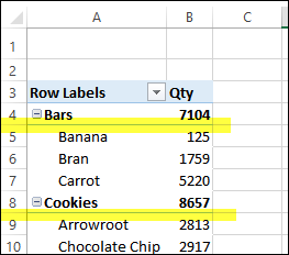
When you create a pivot table, Excel applies a default pivot table style. If there are two or more fields in the Row Labels area, you might see dividing lines, below the item headings.

Those lines separate the items from the heading, and make it difficult to skim through a long pivot table.

Add Blank Lines

A quick fix is to add a blank row after each section:

• Select one of the pivot table headings
• On the Ribbon, click the Design tab
• Click Blank Rows, then click Insert Blank Line After Each Item.

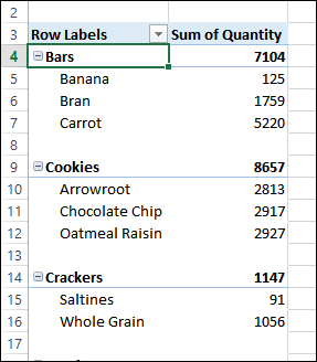
Here’s the result – it’s easier to read, but the pivot table is longer.

Create a Custom Style

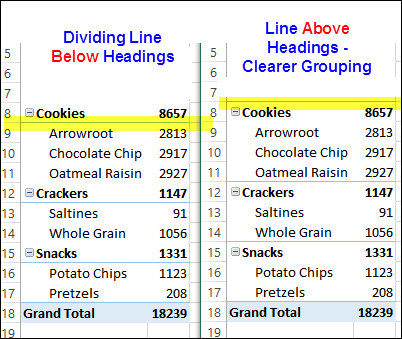
If you’d rather not add lots of blank rows to your pivot table, you can create a custom pivot table style, and change the line placement. In the pivot table on the right, in the screen shot below, I’ve created a custom style based on the original style.

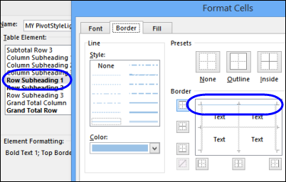
In the new style, the Row Subheading 1 element has the bottom border removed, and a top border added.

Visit my Contextures website for more pivot table style tips.

Video: Better Format for Pivot Table Headings

Watch this video to see how to see how to add the blank rows, or create a new style.