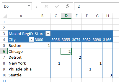
Usually you can only show numbers in a pivot table values area, even if you add a text field there. In the screen shot below, the Max of Region ID is in the Values area.
Instead of the numbers 1, 2 or 3, we’d like to see the name of the region – East, Central or West.

Show Text With Custom Number Formats
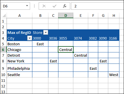
To show text, you can combine conditional formatting with custom number formats. This works well, in Excel 2007 and later, if you don’t have too many text options. In this example, there are 3 regions — East, Central and West.
In the screen shot below, the formula bar shows a 2, which is the ID number for the Central region. The selected cell – D6 – shows the text “Central” instead, because of the custom number formatting that has been applied.

Video: Show Text in Values Area
Watch this video to see how to see how to set up the formatting so text shows in the values area.
Download the Sample File
To download the sample file, please visit my Contextures website. On the Sample Files page, go to the Pivot Tables section, and look for PT0036 – Show Text in Pivot Table Values Area. The zipped file is in xlsx format, and does not contain macros.
_____________

Great tip. I think its works fine without the square bracket arguments either.
What if the Text in Pivot Table Values Area is not something that can grouped at all? For instance the pivot table values are employee’s name, and each of the name is unique?
Unfortunately, a pivot table won’t be able to help in that situation.
Bummer. 🙁
Hi,
Adding Text in place of Number works for 1st 3 values, kindly share some working examples for n number of values and individual text reflecting in the value area against it.