Find the Source Data for Your Pivot Table

After you create a pivot table, you might add new data, or change the existing data. When you refresh the pivot table, it might not show all the new records, or pick up the changes.

To find the problem, you can check the pivot table’s data source. It might not include all the rows, and you’ll have to adjust it.

Video: Find and Change Pivot Source Data

This short video shows the steps to find and change the source data for a pivot table. There are written steps below the video.

Find the Source Data

Follow these steps, to find the source data for a pivot table:

Select any cell in the pivot table.
On the Ribbon, under the PivotTable Tools tab, click the Analyze tab (in Excel 2010, click the Options tab).
In the Data group, click the top section of the Change Data Source command.

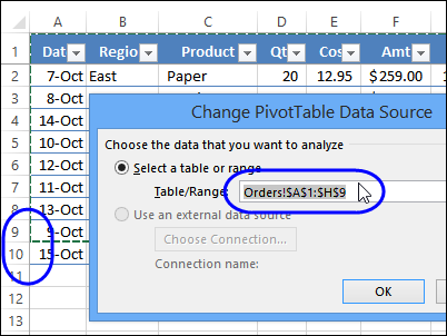
In the Change PivotTable Data Source dialog box, you can see the the source table or range in the Table/Range box. This may be a worksheet reference, such as

Orders!$A$1:$H$9

or a table name, such as

Sales_East

On the worksheet, behind the dialog box, you can see the source range, surrounded by a moving border.

Adjust the Source Data Range

In the screen shot above, you can see that the source data range ends at row 9, and new data has been added in row 10. Because the source data is a specific range – not a dynamic range or named table, it does not adjust automatically when new data is added.

You can adjust the source range, so it includes the new data, but a better solution is to create a table or dynamic range, and base the pivot table on that.

If you want to adjust the source range:

In the Change PivotTable Data Source window, type the new ending row in the range reference
Click OK, to close the window.

This will be a short term solution – you will have to adjust the range later, if more data is added, below the current range.

Use a Dynamic Source

A better solution is to create a dynamic range, based on a formatted Excel table, or using an INDEX or OFFSET formula.

In Excel 2007 and later, you can format a list as a Named Table, and use that as a dynamic source for your Pivot Table. There are instructions here: Excel Tables — Creating an Excel Table. This is a quick and easy way to create a dynamic range, as you can see in the video below.

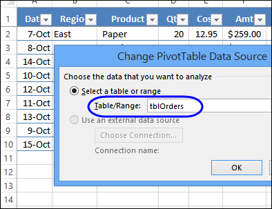
Then, go back to the Change PivotTable Data Source window, and type the dynamic range name in the Table/Range box, and click OK.

In this example, I’ve named the table as tblOrders, so that’s what I’ll enter as the pivot table source.