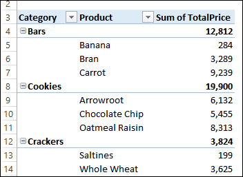
When you set up a pivot table, the outer field names each appear once, at the top of the group. In the screen shot below, The category names are in the left column, and the products for each category are listed below the headings.
Show Repeating Labels
In Excel 2010, and later versions, you can change a pivot field setting, to show the field names in every row, instead of just once. This is useful if the the lists are long, and you can’t see the headings as you scroll down. You can also do lookups from the pivot table, if the names are filled in.
To change the setting:
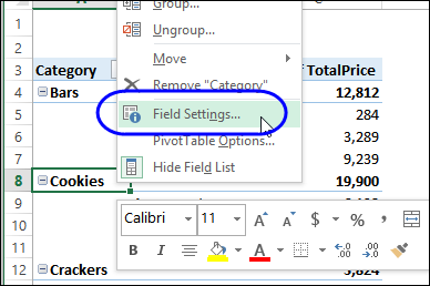
Right-click one of the items in the field – in this example I’ll right-click on “Cookies”
In the pop-up menu, click Field Settings
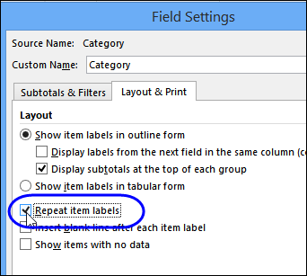
In the Field Settings window, click the Layout & Print tab
Add a check mark to Repeat Item Labels, and click OK
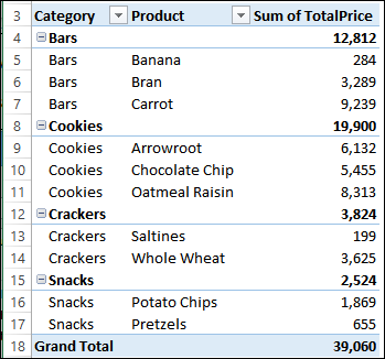
Now, the Category names appear in each row.
Use the PivotPower Premium Commands
If you’ve bought a copy of my PivotPower Premium add-in, you can quickly turn this setting on or off. You can also set this as one of your preferences, in the PPP default settings window.
To apply the setting:
- Select a cell in the pivot field that you want to change
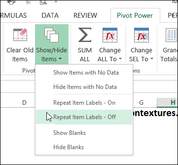
- On the PIVOT POWER Ribbon tab, in the Pivot Items group, click Show/Hide Items
- Click Repeat Item Labels – On or Repeat Item Labels – Off
To set the Default Setting:
- On the PIVOT POWER Ribbon tab, in the Formatting group, click Set Defaults
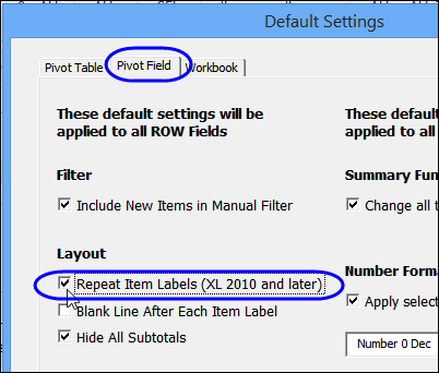
- In the Default Settings window, click the Pivot Field tab
- Add or remove the check mark for Repeat Item Labels (XL 2010 and later)
- Click OK, to save the setting.
__________________
