Apply Multiple Filters on a Pivot Field

Instead of looking at all the data in a pivot table, you can use filters to narrow your focus. See how to apply one filter, or apply multiple filters on a pivot field, without clearing the other filters.

Report Filters

The most noticeable pivot table filters are the Report Filters at the top of the pivot table. You can use those to select one item, or multiple items, to show in the results.

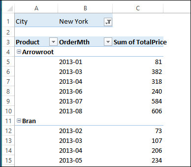
In the screen shot below, the Report Filter has been set to show only New York City. In the Row area, the Product and OrderMth fields have been added, and Total Price is in the Values area.

Filter the Row Fields

You can use filters in the Row and Column fields too. There are 3 types of pivot field filters:

1. Label
2. Value
3. Manual

We’ll see how they work individually, and then how they can be used together.

1) Apply a Label Filter

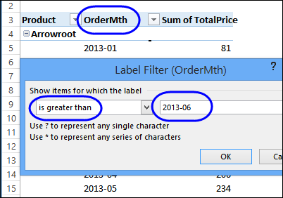
In this example, the pivot table has data from 2013-01 to 2013-12. To show only the last six months of the year, you can use a Label Filter on the Order month field.

• Click the arrow in the OrderMth heading
• Point to Label Filters
• Click Greater Than
• In the Label Filter window, type 2013-06 in the second box, and click OK

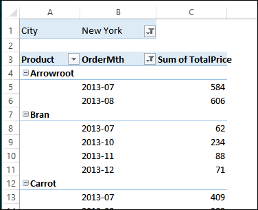
Now, only the data from July to December is visible.

2) Apply a Value Filter

Next, we’ll apply a value filter on the OrderMth field, to show the top 2 months for each product. To do this, we’ll apply a Top 10 filter on the field.

• Click the arrow in the OrderMth heading
• Point to Value Filters
• Click Top 10
• In the Top 10 Filter window, type 2 in the middle box, and click OK

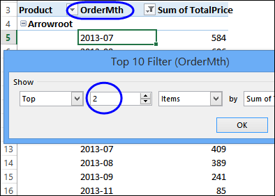
The pivot table now shows the 2 months with the highest sales, but the Label filter was removed. In the screen shot below, month 2013-05 is included in the Bran results. For Chocolate Chip, both months are in the first half of the year.

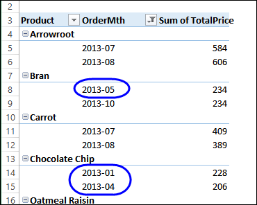
So, when you add a different type of row filter, the first filter is removed.

3) Add a Manual Filter

Finally, we’ll try a Manual Filter. For this, you add or remove check marks in the list of pivot items for the field.

Tip: You can type in the search box, to find items for manual filtering

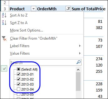
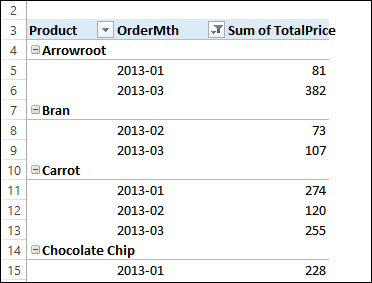
Again, as soon as a new filter is applied, the old filter is removed. Now only the sales from the first 3 months are shown.

Change Pivot Table Filter Options

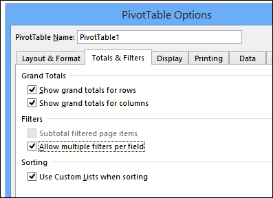
By default, a pivot table is set up to allow only one filter per field, as we saw in the examples above.

However, if you want to use more than one filter per field, you can change one of the Pivot Table options.

• Right-click any cell in the pivot table, and click PivotTable Options.
• Click the Totals & Filters tab
• Under Filters, add a check mark to ‘Allow multiple filters per field.’
• Click OK

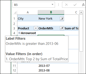
Now you can apply both a Label filter and a Value filter to the OrderMth field, and both will be retained. In the screen shot below, both the Label filter (Greater Than 2013-06) and the Value filter (Top 2) have been applied, and both are in effect, as you can see in the popup message.

NOTE: You’re limited to one of each filter type per pivot field.

Watch the Pivot Table Filters Video Tutorial

To see the steps to apply multiple filters on a pivot field, watch this short Excel video tutorial.

____________