Grouping Shows Items Before and After Date Range

When you group a date field, Excel automatically creates creates groups for all the dates before the start date and after the end date. These items start with a “<” or a “>” symbol, such as “<2012-01-01” and “>2013-12-31”

Usually, you will only see these dates in the filter drop downs.

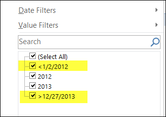
However, if you have the date field to show items with no data, those items might  appear in the headings too.

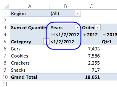
Hide the Out of Date Range Items

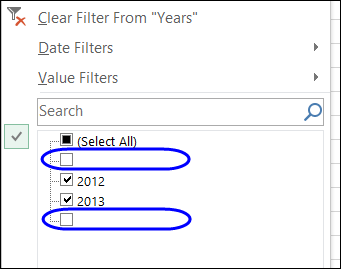
Unfortunately, there’s no setting you can change to prevent these items from appearing in the drop down filter, if you group the dates. However, you could type over the captions, and change them to space characters, so the text isn’t visible.

First, check the date field settings, to make sure that it shows items with no data. This will make the groups appear in the pivot table headings. To check:

1. Right-click on the “Years” field heading in the pivot table, and click Field Settings
2. On the Layout & Print tab, add a check mark to “Show Items with No Data”
3. Click OK

Next, follow these steps to change the pivot item captions:

• On the worksheet, select the pivot table cell with the  “<” date group heading

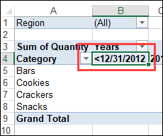
• Type one space character, and press the Enter key

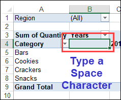
• Next, select the pivot table cell with the  “>” date group heading
• Type two space characters, and press the Enter key

Now you will just see blanks in the filter list, instead of the out of range date labels.

Hide the Pivot Table Headings

To remove the groups from the pivot table headings, change the date field settings, so it does not show items with no data.

1. 1. Right-click on the “Years” field heading in the pivot table, and click Field Settings
   2. On the Layout & Print tab, remove the check mark from “Show Items with No Data”
   3. Click OK

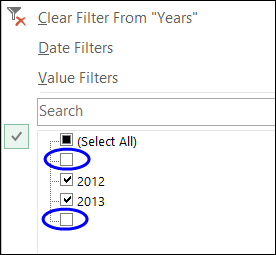
If you need to leave the date field set to show items with no data, you can uncheck the out of date range groups in the date field’s filter list, so they don’t appear in the pivot table.

Macro to Hide Out of Range Dates

Instead of manually changing the grouped date captions, you can use a macro to do the job. The following code works on the first pivot table on the active sheet, and changes the pivot items in the “Years” field.

NOTE: Test this on a backup copy of your file, to make sure it works correctly with your data.

Sub HideDatesOutOfRange()
Dim pt As PivotTable
Dim pf As PivotField
Dim pi As PivotItem
On Error Resume Next

Application.EnableEvents = False
Set pt = ActiveSheet.PivotTables(1)
Set pf = pt.PivotFields("Years")
pt.ManualUpdate = True

For Each pi In pf.PivotItems
   Select Case Left(pi.SourceName, 1)
      Case "<"
         pi.Visible = False
         pi.Caption = " "  '1 space
      Case ">"
         pi.Visible = False
         pi.Caption = "  " '2 spaces
   End Select
Next pi

pt.ManualUpdate = False
Application.EnableEvents = True

End Sub

___________________