It’s easy to create a running total in a pivot table, and it’s usually used to show how quantities accumulate over time.
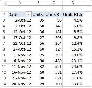
In this example, there are three Value fields in the pivot table, showing the number of units sold on each date.
- In column B, the Sum of Units is shown, with no calculation. This is the number of units sold on each date listed.
- In column C, the Sum of Units is shown, as a Running Total for Date. This is the total units sold, up to and including each date.
- In column D, the Sum of Units is shown, as % Running Total for Date (new in Excel 2010). This is the total units sold, up to and including each date, divided by the grand total of units sold.

Running Total for Date
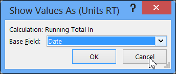
When you select either Running Total In or % Running Total In, you have to select a Base Field. The running totals will be accumulated at each change in that Base Field.
We want a running total down the list of dates, so Date is the Base field in this example.

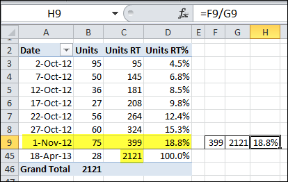
By November 1st, a running total of 399 units have been sold, and the % Running Total is 18.8% of the 2121 overall total units sold.

End of Year Problems
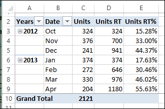
The running total works for a continuous list of dates, but doesn’t flow down the whole list if you group the dates by years and months. In the pivot table shown below, the date has been grouped by Years and Months.
Now the running totals stop at December 2012, and start again in January 2013.

It can be a little difficult to understand the running totals in this layout, so be sure to label the pivot table headings, or add a title to explain it.
______________

I have the task of presenting a pivot chart showing the percentage of jobs correctly closed in an area. The data table shows, for each job, “Y” or “N” depending on whether it has been correctly closed or not. If I present the total counts on the chart using “show values as percentage of row total” it shows percentage “Y” count, percentage “N” count, and percentage total (always 100% obviously). This is more than I want to show. But if I filter the “N”, it does not show me percentage “Y” only, it now shows me “100%”, which is not the required result.
Can you help me understand how to show only percentage “Y”, using either the custom totals or a calculated field?
Debra,
More exploring on this subject led me to your useful article:
https://www.pivot-table.com/2011/03/01/pivot-table-calculated-field-tasks-per-hour/
that confirms I’m not missing something: pivot tables really aren’t well set up to count labels as a percentage of the total, unless I show all the labels. This seems annoying, and an oversight on MS’s part, but at least I can stop looking and just tell my customers that the workaround of helper columns filled with ones is unavoidable.
Hi Debra and Derek,
I am quite new to a more advanced Excel, and therefore would appreciate any help you could provide. I am building an automation for the capacity planning and peerformance for our Enterprise Data Warehouse. I have a source data extracted with SQL from the db, which looks like this (extract):
DT SCHEMA USED_GB
1/28/2013 DB2EDWP1 698.72
2/25/2013 DB2EDWP1 700.33
3/11/2013 DB2EDWP1 701.41
1/28/2013 GBL-DTL 26,438.08
2/25/2013 GBL-DTL 33,467.89
3/11/2013 GBL-DTL 36,894.36
I added an ApplGroup lookup table and a column appl group to the table above.
DT SCHEMA USED_GB ApplGroup
1/28/2013 DB2EDWP1 698.72 Admin
2/25/2013 DB2EDWP1 700.33 Admin
3/11/2013 DB2EDWP1 701.41 Admin
1/28/2013 OPEDWDT 26,438.08 GBL_DTL
2/25/2013 OPEDWDT 33,467.89 GBL_DTL
3/11/2013 OPEDWDT 36,894.36 GBL_DTL
Lookup table:
SCHEMA AppGroup
DB2EDWP1 Admin
OPEDWDT GBL_DTL
Then I created a pivot table as following:
Sum of USED_GB Date
AppGroup Jan-13 Feb-13 Mar-13
Admin 771.98 789.83 799.73
VVOG 925.74 1,003.42 1,083.21
GBL-DTL 26,438.08 33,467.89 36,894.36
I need to be able to calculate month-over-month % growth for each ApplGroup – I know the formula, but am struggling to make it look right. I did not find a way to do this nicely in the pivot table itself, so tried in the source table, but when created a pivot table again – it added a column with the MOM Growth for every month. Is there a way to add a row to every appl group and have it shown under USED_GB? WHat is the best way of doing this?
Then I will need to come up with the projections based on average, but need to exclude MIN and MAX from the AVE calculations, and then it gets even more complicated.
Is there any way i could get help online via a Webex and screen sharing? Please, please help!
Thanks in advance,
-Ellen
Ellen,
Follow Debra’s instructions above, but don’t use these parameters:
SHOW VALUES AS: “Running Total In”
BASE VALUE: “DT”
…use these parameters instead:
SHOW VALUES AS: “% Difference From”
BASE VALUE: “DT”
BASE ITEM: “(previous)”
That should work for you.
Hi,
I would like to filter items based on the running total column. For instance i would only want to show the dates up untill when the percentage becomes 90%
Let me know if this is possible.
Thanks,
Sami