To extract data from an Excel Pivot Table, you can use the GetPivotData function. Unless you change the default settings, a GetPivotData formula is automatically created if you type an equal sign, and then click on a pivot table data cell, to link to it.
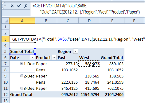
In the screen shot below, I typed an equal sign in cell A3, and then clicked on cell D7, which contains the total sales for:
- Region: West
- Product: Paper
- Date: Dec 1st
The GetPivotData formula that was automatically created is:
=GETPIVOTDATA(“Total”,$A$5, “Date”,DATE(2012,12,1),”Region”,”West”,”Product”,”Paper”)
Replace Text with Cell References
Instead of leaving the text values in the formula, you can replace those values with cell references. This makes the formula flexible, and it will show a different result, based on the values in the linked cell.
For example, I’ve entered a region name in cell A1, a product name in cell B1, and a date in cell C1.
Then, in the formula, I replaced “West” with a link to cell A1, and replaced “Paper” with a link to cell B1.
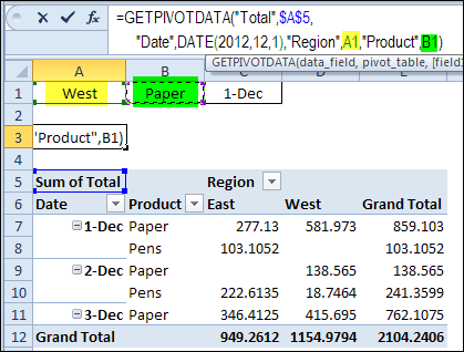
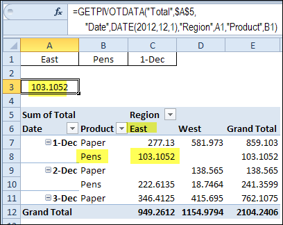
The formula result will now change automatically if I type East in cell A1, and type Pens in cell B1.
Create a Date Cell Reference
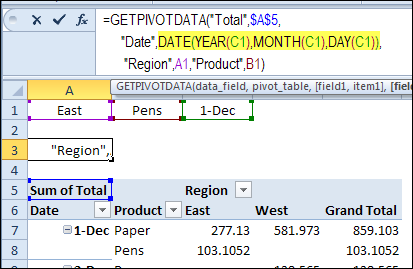
It’s a little trickier to create a cell reference for a date. Instead of just clicking on the date cell, you’ll use cell links within the DATE function.
The arguments for the DATE function are: year, month, day. In the original formula, the selected date is shown as: DATE(2012,12,1)
You can use the YEAR, MONTH and DAY functions to pull those values from the date in cell C1. The completed formula with flexible cell references is:
=GETPIVOTDATA(“Total”,$A$5,
“Date”,DATE(YEAR(C1),MONTH(C1),DAY(C1)),
“Region”,A1,”Product”,B1)
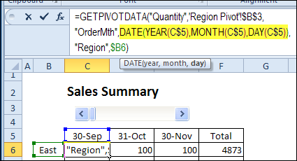
I also used this technique in my Select Date with Excel Scroll Bar example, and you can download a sample file to see how it works.
More on GetPivotData
For more GetPivotData examples, please see my Contextures website: GetPivotData Function
_______________

Great!