In an Excel file, you might have a couple of pivot tables on different worksheets. If you create a pivot chart for one of those pivot tables, you might spend a long time setting it up, with specific formatting and design settings.
It would be nice to copy that chart, and use it for another pivot table, but you can’t alter the source data for a pivot chart.
We’ll take a look at the Data Source setting, and see how you can connect a chart to a different pivot table, by using a workaround.
Pivot Chart Source Data
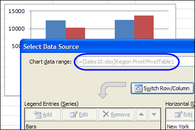
Unlike a normal chart, you can’t change the source data in a pivot chart.
To see the data source for the selected chart, follow these steps:
- On the Ribbon, click the Design tab, under PivotChart Tools
- Click Select Data, to open the Select Data Source window.
In the Select Data Source window, you can see the address of the chart’s data range, but you can’t make any changes to that range.

Unlink the Pivot Chart
So, you can’t directly change the pivot chart source, but with a few easy steps you can solve this problem.
First, follow these steps to make a copy of the chart, and unlink it from the pivot table. That will create a static chart:
- Right-click the pivot chart’s Chart area or border, and then in the popup menu, click Copy.
- On the Excel Ribbon, click the File tab, and click New, then create a new blank workbook.
- On the Excel Ribbon, click the Home tab, and click Paste.
Check the Unlinked Chart
To see what happened to the chart, when you unlinked it, follow these steps:
- Click on a series column in the pasted chart
- Look in the Formula Bar, to see the series formula
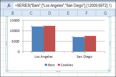
In the Formula Bar, there aren’t any cell references now. Instead, the formula shows text and numbers:
- label names – Bars, Los Angeles, San Diego
- values – 12009, 6972
That’s the result of unlinking the pivot chart from its pivot table.

Link Pivot Chart to Different Pivot Table
Next, you can follow these steps, to link the pivot chart to a different pivot table.
- Right-click the pivot chart’s Chart area or border
- In the pop-up menu, click Cut.
- Switch to the workbook that has the pivot table that you want to use as the chart’s new data source.
- With the chart selected, on the Excel Ribbon, click the Design tab, under Chart Tools
- Click Select Data, to open the Select Data Source window
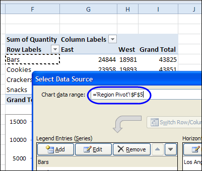
- Click any cell in the pivot table, and click OK

Pivot Chart Linked to Different Pivot Table
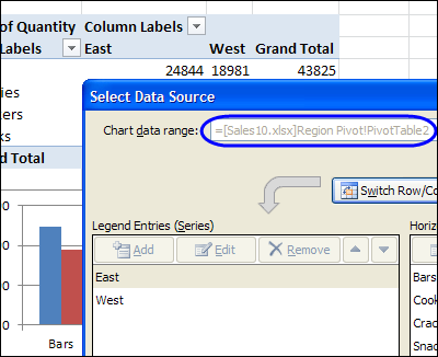
As soon as you make that link to the different pivot table, the static chart changes back to a pivot chart.
To check the data source, open the Select Data Source window again
In that window, you’ll see the dimmed-out reference to the new pivot table.

Watch the Change Data Source Video
To see the steps for changing a pivot chart’s data source, watch this short video.
Get the Workbook
To get the Excel workbook for this article, go to the Excel Pivot Chart Source page on my Contextures site.
The zipped Pivot Chart Source Data workbook is in xlsx format, and does not contain any macros.
___________________________

Very handy, Debra. I didn’t know you could do this. Previously I’ve been saving the old pivotchart as a chart template, then creating a new chart from that template for the new pivot.
Hello!
Thanks for the tip…it’s long winded but better than refromating everything…not sure why it doesn’t let you copy a sheet with a pivot table and chart and automatically link it in the to the new pivot table…used to work in the previous versions…they’ve really messed it up…
I tried it and unfortunately it works only from excel to excel. But it does not work if you have copied a pivotchart in powerpoint presentation, and want to change its datasource.
The chart in powerpoint stays linked to the original pivot table in Excel even if you copy it in a new powerpoint presentation. This is very frustrating because I have spent a lot of time in formatting the powerpoint and now cannot unlink the pivotcharts.
Can someone help?
It does not preserve the exact same formatting in the Chart. It dropped my Data Labels and put Markers on all the line series, none of which resemble the original chart.
I just discovered/created a new and easy way. Copy the original Pivot table (Data source) to a new location, maybe on the same sheet. Delete the original pivot table. This will free up the Pivot Chart to allow you to link to a new data source. Right click on the pivot chart, select “select data, then click in the “Chart Data Range” to create your data source. This should do the trick. You can also copy the original pivot table back in the same location and modify it. You may adjust the pivot table based on how many copies you’ve made.
This article is very useful. thank you for sharing.
Hi, thank u for ur videos, unfortunately I wasn’t able to do it. When i cut and paste it still says pivot chart tool