Change Number Format in Pivot Chart

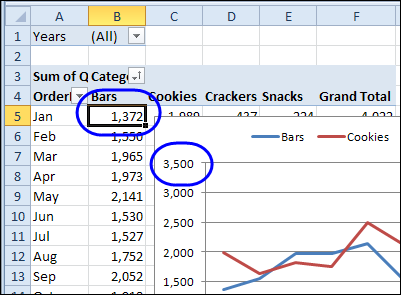
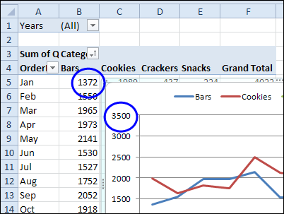
When you create a pivot chart from a pivot table, the numbers on the chart’s axis are in the same format as the pivot table’s numbers. In the screen shot below, the numbers are in General format, with no comma and no decimals.

Video: Change Pivot Chart Number Format

This short video shows how to change the number format for the pivot chart only, or change the number format for both the pivot chart and the pivot table. There are written steps below the video.

Change Pivot Table and Chart

To change the number format in both the Pivot Table and the Pivot Chart, you can change a setting in the pivot table value field. For example, if you want to add a comma separator, follow these steps

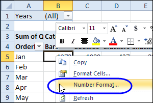
1. In the pivot table, right-click on a cell in the value field. In this example, the Quantity field is in the Values area.
2. In the popup menu, click Number Format
   • 
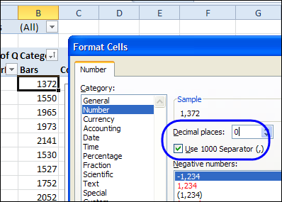
3. In the Format Cells dialog box, click the Number category
4. Change the number of decimals to 0, and add a check mark to Use 1000 Separator.
   • 
5. Click OK, and the number format is applied to both the pivot table and the pivot chart.
   • 

Use Different Number Format in Pivot Chart

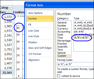
In some cases, you might want a different number format in the pivot chart, rather than making it the same as the pivot table. In this example, you’ll format the pivot chart to show the numbers as thousands, so the numbers take less room.

Follow these steps to change the pivot chart number format, without affecting the pivot table:

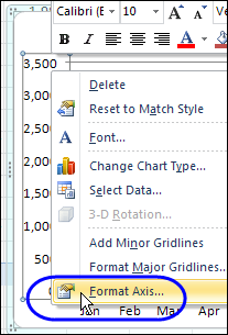
1. In the pivot chart, right-click a number in the axis, and then click Format Axis.
   •     
2. In the Format Axis dialog box, click Number, in the list at the left.
   • 
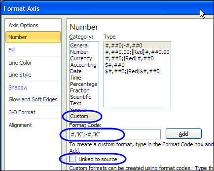
3. Click the Custom category. This automatically removes the check mark from Linked to Source, which disconnects the axis labels from the formatting in the pivot table.
4. In the Format Code box, type a code for the formatting, such as: #,”K”;-#,”K”
5. Click Add, to create the custom number format code, and to apply the format. Only the pivot table has changed – the pivot table numbers are sill in the previous format.
   • 
6. Click Close.

_________________