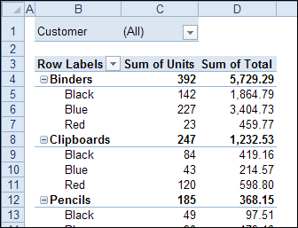
A pivot table shows a summary of the source data, and in the screen shot below you can see all the products that were sold, and the quantities for each colour.

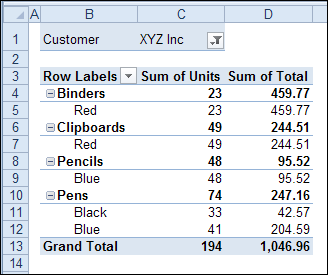
When you filter the pivot table, some of that data might disappear. For example, in the pivot table shown below, the Customer field has been filtered to show XYZ Inc. orders.
They didn’t order all the colours for each product, so the pivot table is smaller. It’s only showing the products and colours that XYZ Inc. ordered.

Instead of having the pivot table change size, so it shows only the applicable items, you can change a field setting, to keep it consistent.
Show All Items in Excel 2010
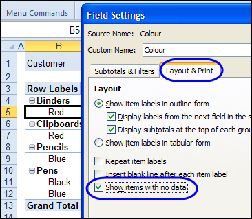
To make all the items appear, even if the pivot table is filtered, you can change a Layout setting in the pivot table. This setting applies to a single field, so you’ll have to make the following change to each field in which you want to see all the items.
To show all items for a pivot field in Excel 2010 or 2007:
- Right-click an item in the pivot table field, and click Field Settings
- In the Field Settings dialog box, click the Layout & Print tab.
- Check the ‘Show items with no data’ check box.
- Click OK

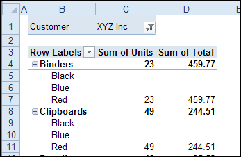
After the setting is changed, all the colours are listed for each product, even if they weren’t sold for the selected customer.

To see the instructions for changing the setting in Excel 2003, please go to my Contextures website: Pivot Table Field Settings
Watch the Video
Watch this video to see the steps for changing the layout setting in Excel 2010 or 2007.
_____________________
