One of the most useful new tools in Excel 2010 is the Excel Slicer. Add a Slicer to the workbook, and you can filter multiple pivot tables with a single click. Here is a warning for Excel 2010 Slicers though, and if you use the Drill to Details feature
Excel Pivot Table Slicers
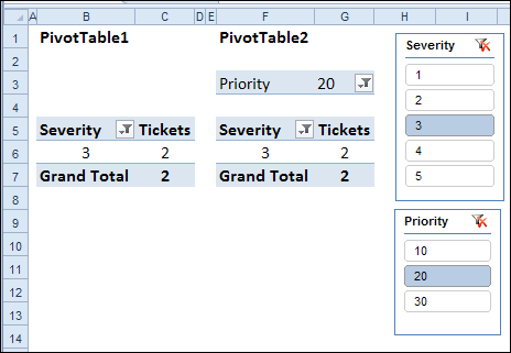
In the screen shot below, there are Slicers for the Severity and Priority fields, and they are filtering both pivot tables.

Drill to Detail
In the worksheet shown above, if you double-click on cell G6, it activates the pivot table’s Drill to Detail feature.
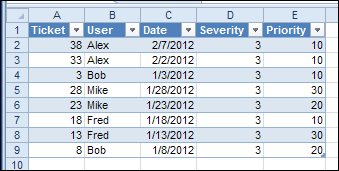
A new sheet is inserted in the workbook, and it shows the two records that have Severity level 3, and Priority level 20.

Warning For Excel 2010 Slicers
However, if you double-click on cell C6 – which also shows 2 tickets – the detail list has 8 records. All of the Priority levels are included, not just the “20” priorities.

This happened because the Priority field is not included in the PivotTable1 layout.
Only the fields in the layout are filtering the data when you double-click to drill to the details.
Use Caution with Slicers
I hope this problem will be fixed, and you’ll see the expected records when drilling to details, even if the Slicer fields are not included in the pivot table layout.
In the meantime, keep this warning for Excel 2010 Slicers in mind, if you’re filtering with Excel Slicers and using the Drill to Details (Show Details) feature.
To prevent unexpected results, add all the slicer fields to the pivot table layout. You could put them in the Report filter area, and even hide those rows if you don’t need to see them. That should ensure that the details list includes only the expected records.
Watch the Drill to Detail Video
To see the steps for connecting multiple pivot tables to a slicer, and the Drill to Detail problem, watch the short tutorial video below.
_______________________
