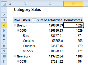
In Excel 2010, there is no built-in summary function that calculates a distinct count or unique count in a pivot table. In the pivot table shown below, we’d like to see the number of stores in Boston, where each product category was sold.
No Unique Count in Pivot Table
Instead of a unique count, this pivot table is counting each record that has a store number. So, the result is really a count of the orders, not a count of the unique stores.
Pivot Table Data Workaround
As a workaround, you can add a column to the pivot table source data, and use a formula to calculate one or zero in each row. In the screen shot below, I used the COUNTIFS function, which is available in Excel 2007, and later versions. In earlier versions, you can use SUMPRODUCT to create a unique count formula.
With this formula, we count the instances where the Order Date matches the current row date, and the Store number matches the current row number, starting from row 1, and down to the current row.
=IF(COUNTIFS(B$1:B2,B2,E$1:E2,E2)=1,1,0)
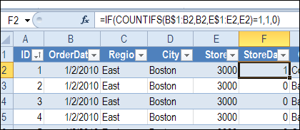
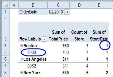
When we add this new field, StoreDate, to the pivot table values area, it shows the correct store count, for the selected date.
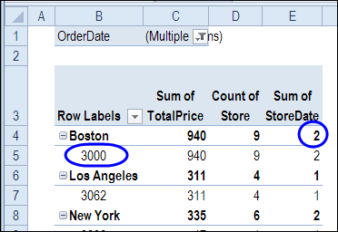
However, if we select more than one date, the StoreDate field no longer shows the correct number of unique stores.
Unique Count in PowerPivot Pivot Table
If you are using Excel 2010, you can calculate a unique count by using the PowerPivot add-in.
- In a blank workbook, use PowerPivot to connect to the workbook that contains your data, and build a pivot table.
Next, you’ll add a new measure to the pivot table, similar to a calculated field in an Excel pivot table.
- Select a cell in the pivot table
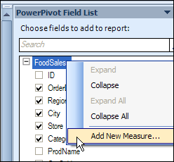
- Then, in the PowerPivot Field List, right-click on the table name, and click Add New Measure
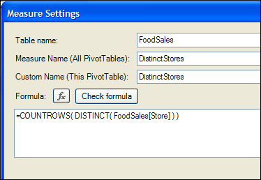
- Type a name for the measure that you are creating. In this example, the measure is named DistinctStores
- Type the formula, to count the rows with a distinct store number. Use the table name and field name – FoodSales and Store in this example
- =COUNTROWS( DISTINCT( FoodSales[Store] ) )
- Click OK, to close the Measure Settings dialog box
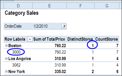
The new measure is automatically added to the PowerPivot pivot table. In the screenshot below, you can see that it is correctly calculating one store in Boston. The StoreCount field is showing 7, which is a count of the orders, not the stores.
Change the Pivot Table
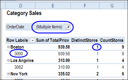
Even if we select multiple dates in the Report Filter, the Distinct Stores field continues to show the correct unique store count.
With the distinct count formula, you can even change the layout, and the results are automatically updated.
In the screenshot below, the product category has been moved to the Rows area, and you can see the number of unique stores where Bars were sold.
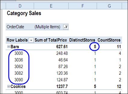
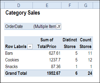
In another layout change, the Store number field is removed from the Rows area, and the unique count is still correct, showing 5 stores selling Bars.
The Grand Total row shows that there were 6 unique stores overall.
Change the Measure Formula
If you have a problem with the Measure formula, you can go back and change it.
- In the PowerPivot Field List, right-click on the Measure name, and click Edit Formula.
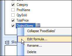
- Make your changes to the formula, then click OK
Video: Show Distinct Count in Excel 2013 With PowerPivot
To see the steps for setting up the pivot table, and creating the formula, please watch this video.
Video: Count Unique in Excel Pivot Table
In this short video, I show how to count unique items (distinct count) in a Microsoft Excel pivot table. This method works in Excel 2013 and later versions.
___________________

Incidentally, in PowerPivot V2.0 there’s a DistinctCount function that does the same thing, so there’s no need to use CountRows(Distinct()): http://technet.microsoft.com/en-us/library/gg492142(v=sql.110).aspx
Thanks Chris, that’s good to know.
Unfortunately, you didn’t show how the fomula changes going down the column. So, I can’t figure out why your example doesn’t work.
KMS, you just copy the formula from the first cell you put it into, all the way down the column. Excel will automatically update the references for you.
Row labels will have 3 fields but i need to move to columnwise …is it possible in xlsx
Thanks a million for this!!!…the formula worked#Appreciative
Awesome…
Is there any way to do get a unique count without Excel 2013, *without* powerpivot add-in, and without the source data in the book?
I use external data sources and create pivot tables directly from the connection, so there is no table (in the workbook) for me to add a column to. We use this method because we are pivoting 250,000 – 600,000 rows of data at a time.
Yes, you can create an OLAP source (with SQL Server Analysis Services or other providers) and bind your pivot table to it. Most of them support Distinct Count measures and dozen of other useful features. Though this requires additional setup, perhaps quite complex.
Yes, it’s described in the second answer at this link: http://stackoverflow.com/questions/11876238/simple-pivot-table-to-count-unique-values
Thank you very much!
You were a great help.