Repeat Pivot Table Labels in Excel 2010

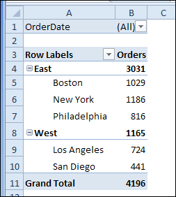
When you create a pivot table in Excel 2010 or Excel 2007, the row labels are in a compact layout – all the headings are listed in column A.

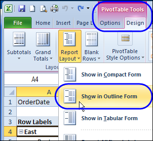
You can change the Report Layout setting, to either Outline form or Tabular form, so each row field is in a separate column.

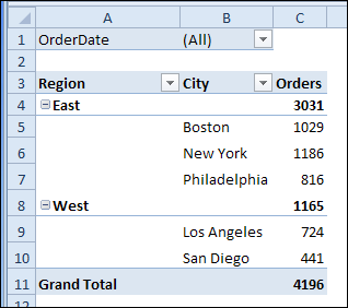
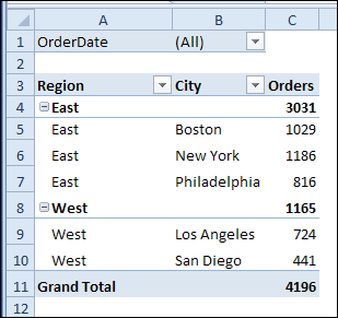
Here’s the same pivot table in Outline form. The Region field is in column A, with a separate row for each new heading.

Repeat the Row Labels

A new feature in Excel 2010 lets you repeat those row labels, so they appear on every row in the pivot table.

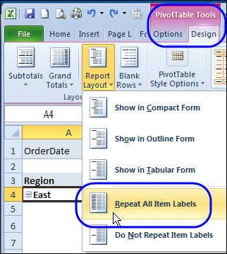
To turn on that feature for all the fields, select the Repeat All Item Labels on the Ribbon’s Design tab.

Here’s the pivot table in Outline form, with repeating row labels.

Repeating Labels for a Single Field

Instead of turning on repeating labels for the entire pivot table, you can apply the feature to a specific pivot table field.

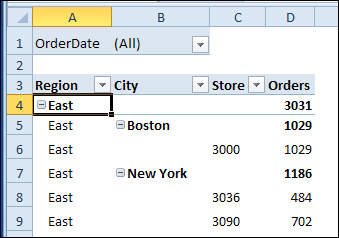
In this example, the Region, City and Store fields are in the Row area, and we’ll turn on repeating labels for the Region field only.

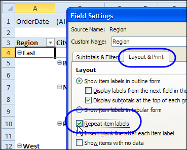
1. Right-click one of the Region labels, and click Field Settings
2. In the Field Settings dialog box, click the Layout & Print tab
3. Add a check mark to Repeat item labels, then click OK

Now, the Region labels are repeated, but the City labels are only listed once.

Watch the Pivot Table Repeat Labels Video

To see the steps for repeating labels in all fields, or a single field, please watch this short Excel pivot table video tutorial.

_________________