Pivot Table Calculated Field: Tasks Per Hour

Instead of creating formulas in the source data for your pivot tables, you can create formulas in the pivot table, by using calculated fields and calculated items.

In this example, we’ll create a calculated field, to show the number of tasks per hour that are completed by each worker.

The Pivot Table Source Data

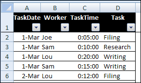
In the source data, each record has the task date, worker name, minutes spent on the task, and the task name.

The Calculated Field Formula

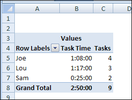
In the pivot table, the following fields are added to the layout:

• worker name is in the Rows area
• Sum of Task Time is in the Values area, formatted to show hours, minutes and seconds
• Count of Task is in the Values area

To calculate the tasks per hour, you would divide the number of tasks, by the TaskTime multiplied by 24.

=Tasks/(TaskTime*24)

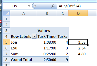
If you wanted to calculate the tasks per hour on the worksheet, outside of the pivot table, the formula in cell D5 would be:

=C5/(B5*24)

The Calculated Field Problem

In a pivot table, you can summarize data by Sum, Count, Average, and several other functions. However, when you create a calculated field, the SUM of the fields are used in the calculation, even if another summary function, like COUNT, is used in the pivot table.

In this pivot table, the Sum of Tasks will always be zero, because Tasks is a text field, and the numeric value of a text entry is zero.

You can read more about calculated fields and calculated items, and their limitations, on my Contextures website.

Add a Task Count Field

Instead of using a text field to count the tasks, you can add a numeric field to the pivot table source data. In the screen shot below, you can see the new field — TaskCount — and a 1 has been added in each record.

To show the new field in the pivot table:

• Change the data source, to include the new column
• Refresh the pivot table
• Remove the Count of Task field
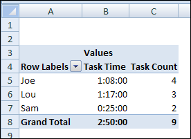
• Add the TaskCount field, as Sum of TaskCount, in the Values area.
• (optional) Change the heading for Sum of TaskCount to “Task Count”

Create a Calculated Field for Tasks Per Hour

To create a calculated field,

• Select a cell in the pivot table
• On the Excel Ribbon, click the Options tab, under PivotTable Tools
• Click Formulas, and then click Calculated Field

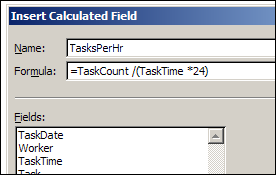
In the Insert Calculated Field window:

• Type a name for the calculated field, e.g. TasksPerHr
• In the formula box, enter the following formula (double-click on the field names to add them to the formula):
• = TaskCount/( TaskTime*24)
• Click OK, to complete the calculated field.

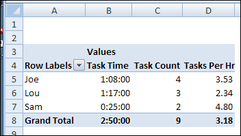
In the pivot table,

• format the TasksPerHr field with the number format that you want, e.g. 2 decimal places,
• (optional) change the column heading.

Video: Create Pivot Table Calculated Field

In a pivot table, you can create your own calculated fields. In this video’s example, I show how to calculate each salesperson’s bonus, based on their total sales.

Download the Sample File

To see the pivot table and formulas, you can download the Pivot Table Calculated Field sample file. It is in Excel xlsx format, and zipped.

You can read more about calculated fields and calculated items, and their limitations, on my Contextures website.
____________