One of the benefits of using an Excel pivot table to analyze your data, is that you can use filters to focus on a specific part of the summarized results. Hiding some of the data with filters can be misleading though, if you can’t tell that filters have been applied.
If you apply a filter in Excel 2007 or Excel 2010, the filter drop down changes to a funnel, with a tiny arrow. In the screen shot below, the ItemSold field has been filtered, to hide some of the items.

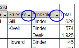
In Excel 2003, and earlier versions, if you apply a filter to a pivot field, the drop down arrow doesn’t change. The same filter was applied in Excel 2003, in the screenshot below, but both drop down arrows are the same.

Create Your Own Filter Markers
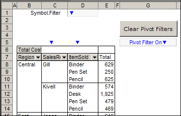
If you’d like to make it easier to tell which fields are filtered, you can use the Excel VBA code created by AlexJ, which displays a bright blue marker above each filtered field.

Download the Sample File
To test the pivot table filter markers, and see the VBA code, you can download AlexJ’s sample file from the Contextures website. On the AlexJ Sample Files page, go to the Pivot Tables section, and look for: PT0000 – Pivot Table Filter Markers
__________
