In recent blog posts, we’ve looked at the pivot table Count function and the Average function. Now we’ll look at two more functions, that are closely related — Min and Max.
Max Summary Function
The Max summary function shows the maximum value from the underlying values in the Values area. The result is the same as using the MAX function on the worksheet to calculate the maximum of the values.
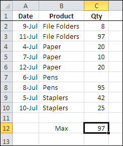
In the screen shot below, you can see the source data for a small pivot table, and the maximum quantity, using the worksheet’s MAX function, is 97.

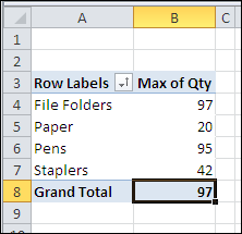
With a pivot table, you can quickly see the maximum for each product that was sold, and the grand total — 97 — which matches the worksheet maximum.

Min Summary Function
The Min summary function shows the minimum value from the underlying values in the Values area. The result is the same as using the MIN function on the worksheet to calculate the minimum of the values.
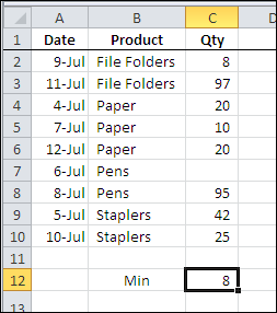
In the screen shot below, you can see the source data for a small pivot table, and the minimum quantity, using the worksheet’s MIN function, is 8.

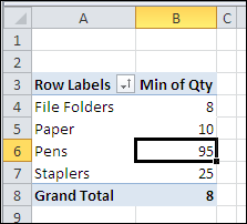
With a pivot table, you can quickly see the minimum for each product that was sold, and the grand total — 8 — which matches the worksheet minimum.

In both the worksheet and the pivot table, the blank cell is ignored when calculating the minimum amount.
___________
___________

Hi Debra. Maybe you can help me with this.
I’m using both MAX and MIN functions in a pivot table to know the older and newest dates for a given row field, and they work fine. The problem is that I want to know the diference between MAX and MIN, but I can’t do it.
I’m trying with a calculated fiel with this formula:
=MAX(Date) – MIN(Date), but it don’t seems to work.
So, if I use both MAX and MIN, how can I get the diference between both of them?
Thanks in advance!
Leonel, a pivot table calculated field will always work on the sum of the underlying values, even if you’re summarizing by another function, like MIN or MAX. You could use a formula outside the pivot table to calculate the difference.
Hello, I need help extracting transactions based on most recent date of occurrence. Here is a sample data.
User Action Date
—– —— ——–
AAA A 8122010
AAA A 8012010
AAA A 6152010
AAA B 7012010
AAA B 6142010
AAA B 6012010
BBB A 8122010
BBB A 8012010
BBB A 6152010
BBB B 7012010
BBB B 6142010
BBB B 6012010
As you can see user AAA performed an action A on 08/12/2010 which is the most recent activity for this user. User AAA performed action B , the latest was on 07/01/2010. How do I extract rows with the most recent date for the user-activity combination? The output I am expecting is records for each category with the most recent date 8122010. I am using Excel 2003 and tried using subtotls custom MAX. But it doesnt seem to work. Will appreciate your help
Max, if you put User and Action fields in the Row area, and Date in the Data area (as Max of Date) you should get the correct result.
If that doesn’t work for you, what result do you see when you try it?
Debra. Your suggestion worked! Thank you soo much. You cant imagine how much time I saved.. Thanks again!
Hi there,
I’m doing a very basic pivot table and know how to do Min and Max one at a time, but am trying to get them side by side so I can see both the Min and the Max at once. is there a way to do this?
Thanks in advance.
Cheers,
Jen
Jen, in the pivot table field list, drag two copies of the field into the Values area, and make one Min and the other Max.
Is there a way to display the second and third highest / lowest totals as well as just the max and min? In a similar fashion to the SMALL or LARGE functions in a worksheet?
For example, in the first screenshot the second highest value is 95, is there a way to show this in a pivot table? And the third largest value in a separate column, and so on?
Andy, there’s no equivalent to the SMALL or LARGE function in a pivot table.
To filter for top items, right-click on pivot item, then click Filter.
Select Top 10, and change the settings to Top 3 Items.
Andy:
As Debra said, there’s no equivalent to the SMALL or LARGE functions, but you can simulate the RANK function, according to M. Alexander:
http://blogs.msdn.com/b/excel/archive/2010/11/02/add-rank-to-pivottable.aspx
In all cases, you can use formulas outside the pivot table.
Regards.
Thanks for the response I worked out a simple way to simulate LARGE (1,2,3, etc…) by adding the relevant columns to the source data and then adding them as Max summary in the pivot table.
Debra (or others),
I have a Table with 4 columns: name, date, task, result. There are hundreds of names, 20 different tasks, and the result consists of a number between 1 and 100. Participants can do each task as many times as they like, with a maximum of 12 times per year. At the end of the year, the winner is that person with the highest total of points on their 10 best tasks. Best meaning where they scored the most points.
Before, I ran a macro that looped though all names, looking up the best score for each task. Those best scores were then ranked, and the highest 10 were copied to a new table.
Trying to do this with a Pivot Table, I can get the highest score for each task with the Max summary function. Is there a way to pick only the top-10 for each person and have a grand total? I know how to do that outside the pivot table, but was wondering if there is a way to get the results without any manual intervention?
Kind regards, John
Hi I have a problem similar to Jen’s above. I have already created a pivot table where the minimum and maximum are side by side along with the total count. The list involves different employees at different counters selling the exact same item but they each have a unique number. By using the max and min I get a range, however, sometimes because items are transferred between the cashiers the range is sometimes broken. For example John had item numbers 1-50 plus items 121-150 transferred from another cashier. His min would be 1, the max would 150 but the actual count will be 80 (50 first range + 30 second range). Is there away to organize it so it recognizes a break in range (i.e. the next item number minus current is greater than one)? Therefore I would wind up with a pivot table that shows John’s name twice, once for range one and once again for range two. Can this be done with a pivot table or is there any method using VBA? Thanks for any help.
Hello,
I have created a pivot table which lists the minimum for each of the divisions I have. But before the total, it relists all of the minimums (same numbers as listed above for each division but in a different order). How do I remove these extra minimum values?
@Sarah, you might be using a Min Custom subtotal for that field, as well as showing the data summarized by Min.
To remove the custom subtotals:
–Right-click on one of the division names in the pivot table, then click Field Settings.
–Under Subtotals, click Automatic, and click OK
I have 3 items in a pivot that are pulling max amount for each from the data. How do I get the top summary to total the sum of the max items without changing the condition to Sum?
Example:
Currently
Total 4 This is showing the max
Cumbustor 2 (this is max)
Extractor 4 (this is max)
Exhaust 2 (this is max)
Need
Total 8 NEED TOTAL OF MAX
Cumbustor 2 (this is max)
Extractor 4 (this is max)
Exhaust 2 (this is max)
Question, how do you actually locate the first column value of the maximum value? Like the first example you did, the correct result should be “11-JUL”. I tried to use hlookup and max together but it doesn’t work unfortunately.
@Stan, you can use INDEX and MATCH functions to get the value from the first column. There are examples on my Contextures website:
http://www.contextures.com/xlFunctions03.html#IndexMatch
Thank you Debra
Needing your help please…. I need to come up with a formula that will calculate the following:
Oct. 12 Tab
Max YTD: – Cell D: 85,902
Max Date (peak occurred): – Cell E: 10/15/12
Nov. 12 Tab
Current month: – Cell B: 85,011
Date occurred: -Cell C: 11/13/12
Nov. 12 Tab
Max YTD: – Cell D: 85,902
Max Date (peak occurred): – Cell E: 10/15/12
Dec. 12 Tab
Current month: – Cell B: 79,433
Date occurred: – Cell C: 12/3/12
Dec. 12 Tab
Max YTD: – Cell D: 85,902
Max Date (peak occurred): – Cell E: 10/15/12
The Max YTD is a # gathered for the highest peak total (85,902) which Starts at Fiscal Year Oct. 12. This highest peak # took place during Oct. 12 which happened to be on 10/15/12.
I need to come up with a formula that will calculate the following:
I need to take the Max Oct.12 YTD Cell D: 85,902 + Max date Cell E:10/15/12 and the Nov. 12 current month Cell B:85,011 + date Cell C:11/13/12 max these two #s’ and two dates then input new data into Nov. 12 Max YTD Cell D: + Max Date Cell E:
This process keeps reaping each month until end of Fiscal Year Sept. 13
For each month starting with (Oct – Sept) if the Max YTD is greater than (85,902) the new highest peak # has to be carried over to the next month along with the date it occurred and this keeps reapting every month. Even if the Max YTD does not change it still has to be carried over to the next month until end of Fiscal Year Sept.13.
I am working with Excel 2010 and very new at this.
Could you please help me figure out how to get the max of activity period below either in excel or pivot?
Award ID End Date Activity Period
A123456 1/31/2021 01
A123456 1/31/2021 02
A135679 8/31/2022 03
A135679 8/31/2022 04
Thank you,
How to do this when you have a pivot table that keeps wanting to give you a sum-of-values rather than the Mx for that top-10 group?