In a pivot table, there’s no built-in way to group the pivot table data by both weeks and months at the same time. If you want to show sales data by week, you can group the date field in seven-day intervals.
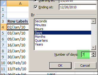
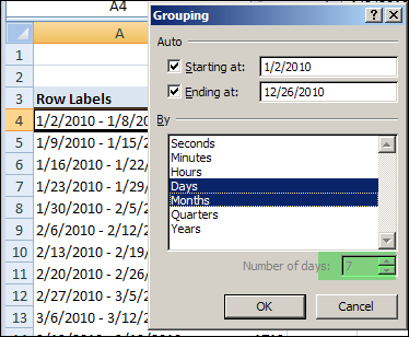
The 7 day grouping works well, but if you try to add grouping by months, the Number of Days option is disabled. If you select Month in the Grouping dialog box, the days will lose their 7 day grouping.
Calculate the Month
Since you can’t group by both week and month, you can use a workaround instead. You could create a column in the source data, and then calculate one of the grouping levels there. Then, you could add that field to the pivot table.
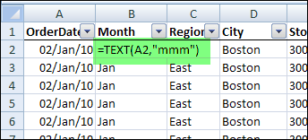
For example, you can add a column that calculates the month name for each sales order date, by using the TEXT function:
=TEXT(A2,"mmm")
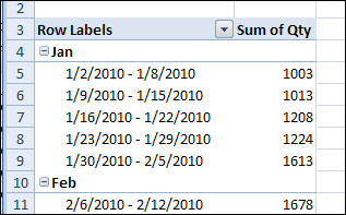
Add the Month field to the pivot table, above the weeks.
Calculate the Week Number
Another option is to add a column to the source data, with a formula to calculate the week number:
=WEEKNUM(A2).
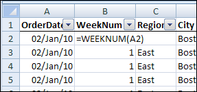
With the OrderDate field in the Row Labels area, group the dates by months. In the Row Labels area, add the WeekNum field below the OrderDate field, to summarize the data by month and week number.
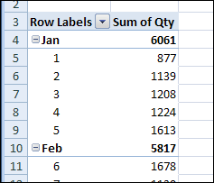
Note: If a week begins in one month and ends in another, it will appear under both months.
________________

I have an ODBC link with a database how can i create weeknumbers.
Now i am using The 7 day grouping it works well, but for a reason i dont know yet sometimes the grouping starts with 16-10-2011 and not with 02-01-2011
thanks