You can create a calculated field in a pivot table, to perform calculations based on the Sum of a pivot table field. For example, the formula below would calculate a bonus based on the total number of units sold for each product.
If 60 or more were sold, then the salesperson would receive a 3% bonus on the sales amount for those products.
=IF(Units>= 60,Total* 3%,0)
The Pivot Table
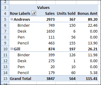
In the pivot table shown below, Andrews sold 150 binders, and earned a bonus of 22.46 on that product. Gill only sold 10 pens, so there is no bonus earned for that.
The headings in the pivot table have been changed:
- Sum of Total –> Sales
- Sum of Units –> Units Sold
- Sum of Bonus –>Bonus Amt

Calculated Field Totals
After creating the Bonus calculated field, you might expect to see a sum of the bonus amounts, in the subtotal and grand total rows. However, the calculated field uses the same calculation in the subtotal and grand total rows, instead of showing a sum.
In this pivot table, Gill had two bonus amounts — 11.98 and 5.38, for a total of 17.36. However, the subtotal for Gill shows a bonus amount of 26.21, which is too high.

The grand total for a calculated field performs the same calculation that’s defined in the calculated field. So, for Gill, instead of summing the bonus amounts, it calculates 3% of Gill’s total sales — 874 * 3% = 26.21
Calculate Outside the Pivot Table
Unfortunately, there’s no setting that you can change in the pivot table, to sum the calculated fields, instead of using the calculated field formula on the totals.
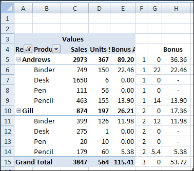
As a workaround, you could use formulas outside the pivot table to extract the bonus amounts, and sum those amounts.
- To create blank cell in the product column, the report layout was changed to Outline Form.
- To create salesperson groups, in cell F5, the formula is: =–(B5=””)+F4
- (Note: there are 2 minus signs after the equal sign in the above formula)
- In cell G5: =IF(B5<>””,E5,0)
- The bonus calculation in cell H5 is:
=IF(A5=”Grand Total”, SUM(G:G), IF(B5=””, SUMIF(F:F,F5,G:G),G5))

Then, hide the pivot table column that contains the Bonus calculations, so only the column with the correct subtotals and grand total is visible.
Video: Create Pivot Table Calculated Field
In a pivot table, you can create your own calculated fields. In this video’s example, I show how to calculate each salesperson’s bonus, based on their total sales.
Download the Sample File
To work with the data in this example, and create the calculated field, you can download the Calculated Field Bonus sample file. The file is in xlsx format, and zipped.
_____________

The workaround would be even better if you use Get Pivot Table Data feauture.
It seems to me that the workaround also assumes that the pivot table is stable. If you have an unknown number of rows, it’s still problematic.
@Paul, you’re right, if the pivot table will change size, you could add the formulas with a macro that runs automatically when the pivot table changes.
A much better solution would be to calculate the bonus amount before creating the pivot table – either in the sql or on the original worksheet. Then everything will show correctly on the pivot table, no matter the changes to the layout.
I find calculated fields are most useful for calculations involving percenatges – e.g. calculating percentage growth. For these problems, calculating the percentage change works, but all the summary information is wrong. That’s because it sums the percentages – not what is wanted. Even using average instead of sum is not helpful, because you usually need a weighted average, not a simple average. Calculated fields work great for these problems for the same reason it caused the problem in the article – for instance, the grand total is calculated using the formula in the calculated field; exactly as desired.
I have following pivot table:
Region Zone #of customers Sales Sales/sub Totals of ZONE
south 1 50 $ 1000
total 1 50 $1000
2 60 $ 1500
total 2 60 $1500
total south 110 $2500
now i want to get a %age sales to the total # of customers in ZONE, which has sub totals 1 & 2.
Can anybody help me and give the solution. My email address is [email protected].
Thanks.
Junaid
Debra – If you still have it, will you attach the file you used for this post as well? (Can you tell I’m focused on calculated fields? :))
Sure Bob, I’ve uploaded the sample file for this post. Hope you’re having fun with the calculated fields!
Corrected link:
I just thought I would post a relevant bug report from Microsoft which seems to explain why this useful workaround is required.
http://support.microsoft.com/kb/211470
Can anyone help with this… I have entered a calculated field to give me a calcuation of Gross Profit % (of total sales and gross profit £) but it is only entered a figure in the total column – really need it by month (all other columns) – anyone help please?…. 🙂
can I have a display option using a pivot table where i need to display only the customers who have not given orders in a particular month amongst the ytd data
Hi
Not sure if this helps but i had a similar problem calculating a £value based on a sumed up stock level (calculated as a demand figure * 2 which i called “Level”) and a cost price. Excel was summing up the costs as well as the qualtities. The solution looks very odd but works.
I added an extra column on my data which just contains 1’s which i called “Line”. This then allowed me to do the following as a second calculated field.
=(Level*(‘Invoice Cost’/Level)/Line)*Level
Hope this is of help
Steve
Appologies, just realised i pasted my first attempt, my someone shortened version is this:
=((‘Invoice Cost’/Line)*Level)
I am having an issue in a pivot table that is showing a correct difference when the calculated change field cell uses a higher headcount less a lower headcount which yields a positive result. However, when the calculated change field cell uses a lower headcount less a higher headcount which would yield a negative number, the result on the pivot table for the calculated change cell is blank. How can I fix this? Thanks
If you check Pivot table Options -> Layout & Format there is a Format option ” For error values show” which is by default to show a blank cell when an error is encountered. It may be that the calculation generates an error when using the lower headcount.
I usually set format to show N/A so I can see any errors easily.