Summarizing Formatted Dates in Excel Pivot Table

If you format a column of dates in your pivot table source data, to show as year and month (yyyy-mm), they won’t automatically summarize by year and month in the pivot table.

Format the Source Data

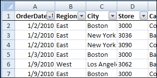
For example, in the source data shown below, there are several orders for January 2010, and three different dates are visible.

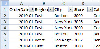
If you format those records as yyyy-mm, it looks like all the dates are the same.

Summarize Formatted Dates

However, when you add the OrderDate field to the Row Labels area of a pivot table, several items appear as 2010-01, instead of only one item.

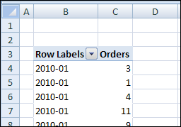
The first instance of 2010-01 shows 3 orders, so that would be the Jan 2, 2010 orders. Below it is an item with a single order, and that’s a summary of the Jan 3, 2010 orders.

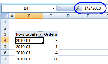
Even though the dates are formatted to look the same in the source data, the underlying dates are still recognized by the pivot table. Those underlying dates are used for the pivot table summary. If you click a date in the Row Labels, you see the underlying date in the formula bar. Because the dates are different, each date is listed individually.

Group the Dates

Instead of formatting, you can group the dates in the pivot table to combine the data by month and year.

1. Right-click an OrderDate row label, and then in the context menu, click Group.

   

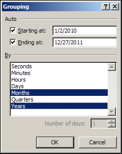
2. In the Grouping dialog box, in the By list, select Months and Years, and then click OK.

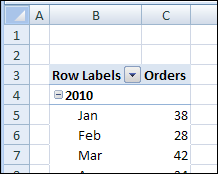
The orders will be grouped by year and month, showing a total of 38 for January 2010.

Calculate the Year and Month

Grouping can cause some problems in a pivot table, such as preventing you from using calculated items. If you don’t want to using grouping, you could add a new column to the source data, and enter a formula that converts the dates to text. Then, all the dates that have the same year and month will calculate to the same text string.

In our example, the order dates are in column A.

1. Add a blank column to the source data table, with the heading YrMth.
2. In the cell below the heading, type the formula =TEXT(A2,”yyyy-mm”)
   
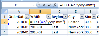
3. Copy the formula down to the last row of data in your table. (Note: If your data is in an Excel Table, the
   formula should fill down automatically.
4. Refresh the pivot table, so you can see the new YrMth field in the PivotTable Field List.
5. Add the YrMth field to the pivot table Row Labels area.
6. Remove the old OrderDate field from the pivot table layout.

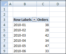
The orders are grouped by year and month, showing a total of 38 for January 2010.

_________________