Remove a Pivot Table Style in Excel 2007

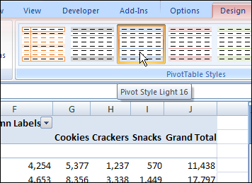
When you create a pivot table in Excel 2007, a default PivotTable style is automatically applied to a pivot table. For example, in the screen shot below, the pivot table uses the Pivot Style Light 16.

Remove the Pivot Table Style

In some workbooks, you might prefer to have a pivot table with no fill color or header formatting.  In the PivotTable Styles gallery, you can apply a special style to remove the existing style.

Follow these steps to clear the PivotTable style:

1. Select a cell in the pivot table.
2. On the Ribbon, click the Design tab.
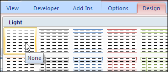
3. In the PivotTable Styles gallery, click the first style, None, at the top left of the Light styles.

Pivot Table Style Removed

After you click the None option, the existing style is removed, and a thin border remains around the pivot table sections. The worksheet gridlines, if displayed, are not visible within the pivot table.

Also, when no PivotTable style is applied, the preview function does not work if you point to a different style in the PivotTable Styles gallery.

Clear the Pivot Table Style

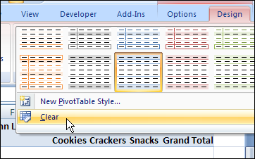
Another way to remove the PivotTable style is to click Clear, at the bottom left of the PivotTable Styles gallery.

______________

For more information on Pivot Tables, please see the Pivot Table Tutorials on the Contextures Website.

______________