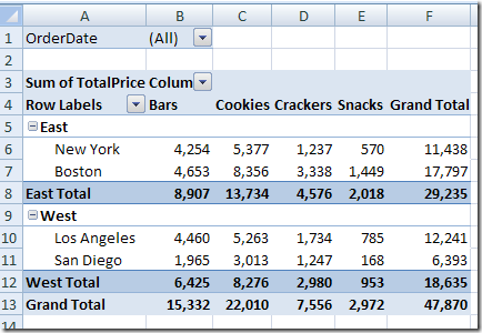
Even though a pivot table is automatically formatted when you create it, you can add your own formatting later. For example, in the pivot table shown below, I’ve added colour to the subtotal rows, and made column B narrow.

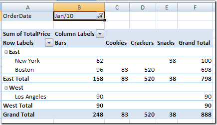
However, some of that pivot table formatting might be lost if you refresh the pivot table or change its layout. Even if you select a different item in the report filter, the formatting could be lost.
Here’s what the same pivot table looks like, after I select an order date from the report filter.
Preserve the Formatting
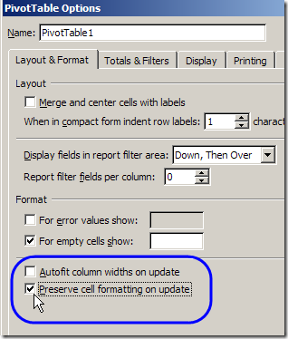
Most pivot table formatting can be preserved if you change the Format options in the PivotTable Options dialog box.
- Right-click a cell in the pivot table, and click PivotTable Options.
- On the Layout & Format tab, in the Format options, remove the check mark from Autofit Column Widths On Update. This will prevent column widths from changing, if you have manually adjusted them.
- Add a check mark to Preserve Cell Formatting on Update
- Click OK.

Apply Formatting
After changing these Pivot Table options, the formatting should stick. When you apply formatting to the Pivot Table, do the following:
- Ensure that Enable Selection is turned on.
- Unless you want to format a single cell, use the pivot table selection technique to select the elements you want to format (point to the top or left edge of the element, and then click when the black arrow appears).
______________
P.S. For more information on Pivot Tables, please see the Pivot Table Tutorials on the Contextures Website.
_________________


DOES NOT WORK!
Does not work. I can’t find any accurate directions to change a number/date format in a pivot chart and have it saved.
This does NOT work. I don’t know why this same ‘solution’ seems to show up on every message board, but it won’t work.
What type of formatting are you applying to the pivot table? What version of Excel and operating system?
This does not work. I’m using Excel 2010, and would love to find a way to preserve the formatting of columns. For instance, I have a time field formatted hh:mm on data list. The pivot displays this as hh:mm:ss. I go through all the steps listed above, but any new data added is in the hh:mm:ss format. My formatting only holds for the previously formatted cells. I cannot find the answer anywhere.
In one of my pivot tables I can’t even get the formatting to hold on previously formatted cells. It works in other files, but for this file if I remove a field and then put it back in, it loses the format. I’ve checked every option I can find, including all those above, and nothing works. I recently converted to Excel 2010, but I think this is a 2007 file. Any ideas?
Agreed, it doesn’t work. I’m on office 2010. My biggest pet peeve is with the borders. If I expand my entire sheet, highlight whole table, then select “No Border” it will remove them. THEN when I collapse and open again, they return everytime, usually in different places. The same is true when I select “All Border” they all disappear except a few blotches of “thick box border.”
I’m so glad I’m not alone – I have been struggling with this for ages, it looks perfect at first, but if you remove a value from the value field and then put it back the formatting is always lost. I create my table for many people to use on a shared data system and it is very frustrating that it can’t simply stick – I only need ‘currency’ and ‘number’ formats to stick for about 6 fields.
Anyone had any luck yet?
I’m finding that the key part is in the ‘apply formatting’ part of the instruction above – i.e. If I change the format by selecting the whole column (eg. E:E) and formatting it like I normally would, it won’t stick. However if I change the format by using the method above – where you click on top of the pivot field till the little arrow comes up, click the arrow so that the pivot cells ONLY in that column are selected, and THEN right click to ‘format cells’ and change the format…. then it sticks upon refresh… woohoo!
tqvm! it works
I don’t have any problem with the format sticking upon refresh. It’s when I take a field out of the values box and then put it back in — I put the field in, format the number, then take the field out. When I put it back in, no formatting. I tried the method above, same problem.
The interesting (and frustrating) part is that this only happens in this workbook. Most of my other workbooks will hold formatting, but I can’t figure out what’s different about this one.
Ok, I found something that has worked so far. I noticed that the default number format for the sheet that the pivot was on was General. I changed it to Accounting (which was what I had been trying to get the pivot table to use), and now I don’t have to format anymore. Go to the Number area on the Home tab and use the drop down box to set the default number format. This doesn’t solve the problem of the pivot table holding formats if you want different formats for different fields, but it works for what I’m doing.
This worked great..I have seen the same instructions about the Enable selection and the Preserve Cell Formatting on other sites. This is the first explanation that included that I needed to select the column with the black arrow at the top. Once I did that the formatting remained upon refreshing the data.
There are a couple of other things you can try. Expand everything before making changes the formatting of the body of the table and turn on Field Headers, make the formatting changes and then turn off Field Headers – then the changes stick. Well, they did at least for me.
This might help.. after doing the procedure above. Select pivottable. Enable all borders. Then disable it. Then change the format to whatever you want. Refresh. Format should stick. It worked for me at least. 🙂
Highlight at cell that is formated the way you want. From the “Home” menu, go to “Cell Styles”. At the bottom of the pop-up menu, hit “New Cell Styles”. Check the items you want to be included in the new cell style. (At this point, I would assume that you would keep all of the items, but you can uncheck some or you can hit the “Format” button and format the cell the way you want. Save this new “Cell Style”. Hightlight the cell or group of cells that you want to apply the new format with the “select arrow”. Go back to “Cell Styles” on the “Home” menu and select the new style you just created. The highlighted cells should now be formated the way you want and they should remain the same after a “Refresh” is done.
I’ve tried all of these suggestions (in Excel 2010) but whenever I remove field and add it back to the PT, it loses its number formatting. I have some fields that require dollar currency and some require Euro currency.
@Sunali, you nailed it! Very subtle the method of selecting a pivot table column while the little arrow is showing, then right-clicking to Format Cells. That did it! Bravo, and thanks!
BTW, selecting while the ‘down arrow’ appears in any cell will select the entire column of data below the column header. Selecting while the ‘right arrow’ appears in any cell will select only that cell.
Does anyone have a suggestion for formatting row heights in pivot tables? After I refresh my data, the row height is too great, causing my printed file to be larger than I would like. Also, the row height is inconsistent, with a greater height for rows at the top of the table and a smaller height at the bottom. Weird. Even though I fix the formatting before I print, and save….every time I refresh the row heights change. This is really annoying! Any thoughts would be appreciated. thanks.
Amy, I have found through trial and error that all filters need to be off before formatting. For instance, if you have any slicers or date filters, remove them so all data shows in the pivot, adjust the row heights, then reapply your filters.
Here is the method that worked for me every time when using a Pivot table with Slicer feature:
1. Create your Pivot table with or without Slicer option.
2. Click on any cell in the body of the Pivot table
3. Click on OPTIONS under Pivot Table tools at the top of the ribbon (the other choice will be DESIGN).
4. Look for FIELD SETTINGS in the ribbon to the left in the Active Field box. Click it.
5. In the Value Field Setting box that opens click the “Show Values As” tab.
6. In the bottom left click on NUMBER FORMAT. Under FORMAT CELL choose your format and click ok.
Once you do the above the whole Pivot table will update to the format you choose. Last step. CLICK SAVE!
Now when you filter, Slice, or Dice the format stays the same.
Moe
The issue with date formats and numbers can be fixed, I got bored readng above so apologies if covered, but you need to change how the source data is put in, if done correctly then it will keep them (my formatting issues are not resolved here, but maybe yours can be helped)
Use for example, instead of a date field being picked up, use a string. for instance a cell may have the data in it formatted in whatever way. you can change this to a string by doing the following..
say you have a date in cell A2, and you’d like to have the format as ddd, dd,mm,yy then in a cell picked up by your pivot, have the following =text(A1,”ddd”)&” “&text(A1,”dd”)&” “&text(A1,”mm”)&” “&text(A1,”yy”)
That will not be changeable by updated refreshes.
best wishes
Paul Turner