A common question is “How can I show text in a pivot table’s values area, instead of numbers?”
For example, if you add the Region field to the Values area, you’d like to see the region’s name, instead of a Count Of Region number.
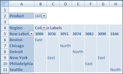
If you use Crosstab queries in Microsoft Access, you might have achieved this by using the First or Last summary function, instead of Sum or Count.
Unfortunately, the First and Last functions aren’t available in Excel pivot tables, so there’s no easy way to show text in the Values area.
Workaround #1 – Use the Row Fields
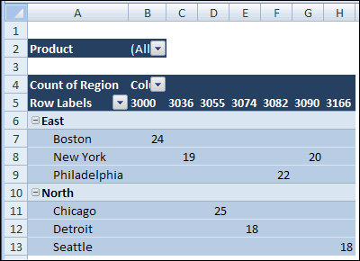
You could add the Region field to the Row Labels area, with the City field. Then add another field in the Values area to show a count of the regions. The layout won’t be exactly what you wanted, but it will show the region name.
Workaround #2 – Create a Custom Number Format
In this example, there are only two region names, so you could use a custom number format to show the region names. You’ll assign a number to each region, then use that number in the pivot table. Note: This technique is limited to 2 items.
Create the Region Number field:
- In the source data, add a new column with the heading RegNum. In this column, type a 1 for East region orders and 2 for North region orders.
- Refresh the pivot table, so the RegNum appears in the Field List.
- Add the RegNum field to the Values area, and right-click on one of the numbers.
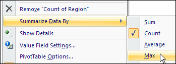
- In the popup menu, click summarize by Max.
Apply a Custom Number Format:
- Right-click a Region value in the Values area in the pivot table.
- In the popup menu, click Number Format.
- In the Category list, click Custom.
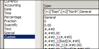
- In the Type box, enter [=1]”East”;[=2]”North”;General
- Click OK, to close the dialog box.
The pivot table will show the Region names, instead of the Region numbers.
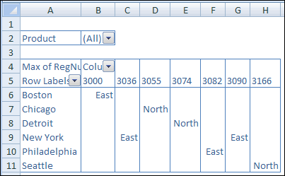
____________

Hi ,
I’ve done this example for 1 and 2 but does it not work up to 3 and 4? Is their a limit?
Thanks
Yes, this is a very limited way, only up to 3.
Hi Mark,
Yes, there’s a limit of 2 items that can be formatted this way with a custom number format. I’ve added a line to the blog post, to clarify that.
Thanks,
Debra
I am unable to use it on large scale. its good with 1 or 2 values. but not with more then 10 values.
But its good thing. THnx
Thansk very much it was a great help
good tip, but useless for x1000 of values
Hi Debra,
Thank You Very much for saving us. This is the only workable way I have found after searching hundreds of web pages.
Any way you can define different set of coding and do the same thing so that the txt fields are appearing.
(Eg; Code 1: for “North” [=1], “South”[=2] code 2 for “East”[=3],”West”[=4])
But the appearance of the table is bit of a issue.
Thilan Balasuriya
Debra,
last year I published a workaround for creating cross tabular views with texts in the value area. Not an Excel Pivot Table, but a VBA routine generating a cross-tab, looking like a Pivot Table (well, more or less). It is not too complicated to implement, even if someone is not familiar with VBA.
You can find the article and the Excel workbook for free download here:
Emulate Excel Pivot Tables with Texts in the Value Area using VBA
After reading your article and the comments here, I thought some of your readers might be interested.
Best regards
Robert
Thanks!
This information saved my day!
Thank you, thank you, thank you!
Hi there,
Just noticed that the solution with the custom formatting also works for CONDITIONAL FORMATTING. This way there do not seem to be limitations as to the number of possible variables (Code 1: for “North” [=1], “South”[=2] code 2 for “East”[=3],”West”[=4]etc.). I’ve got Office 2007 on my computer and it works.
Kr
Luke
Hi , Is this same way to perform for many varialbes as showed in the article.
Luke – Thx – how do you get the CONDITIOANL FORMATTING to remain after you update the table – I loose my formats they return to the prior format?
Thanks for sharing.
It method doesn’t seem to work if ‘1’ and the ‘2’ is formuled.
e.g. In my newly created column in the datasource, I have the formula =if(A1<50,"1","2")
How can I get around this please without having to manually enter in the 1's and 2's?
@Tisha, don’t use the quote marks around the 1 and 2. Change your formula to the following and it should work correctly:
=if(A1<50,1,2)
Hi,
thanks for the info.
probably the following is not the solution for every issue here, but after searching for a while – and telling my boss in not to subtle words that a pivot table is not ment to do this – I found the following procedure for displaying rows of text in my pivot chart without entirly wrecking it:
office2010:
-click the pivot table
-in the ribbon select
“pivot table tools” -> “options” -> “options” (on the far left)
– the menu “pivottable options” opens
– hit the “display” tab
– check “classic pivot table layout (enables dragging of fields in the grid)”
drag the rows next to each other (instead of having them grouped below)
again, not nice, but did the trick for me.
Huge help !! Thank you for these postings!!!
Wow! That was most helpful! Thank you!
You are a life saver!!!
Thanks pdt.
This post was very helpful! I had some trouble with re-arranging the table and it worked with enabling the “classic” layout. Thanks!
It took me some time to work out what Luke said about CONDITIONAL FORMATTING that seems to be the ,best option, as it is not limited. This is how it works (excel 2010) (you need to create a sepperate rule for each value):
Select the cells you want to format in the pivot table,
press CONDITIONAL FORMATTING button on the ribbon, extra rules, format cells equall to, after you have entered the value press FORMAT->customize ->
and type the following text in the type text box:
[=4]”Good”;General
(now create a sepperate rule for each value you want to display)
you can also make it a different color: [=4][blue]“Good”;General
So…in a pinch, I ended up concatenating fields in the data table. This way, when you run your data, the information still gets grouped with the appended data. In my case I was trying to match employee with insurance # and specific account numbers. I concatenated insurance policy numbers with account #’s and grouped by employee nested by insurance type. It’s cheating, but it works and it’s really quick.
make a separate column in your datasource
if YES=1
if NO=0
make a measure in your pivot table, which goes like this
=IF([Column with 0 and 1]=1;”YES”; “NO”)